Chapter 10 The continental United States is similar
As a second replication, earthquake data from the continental United States is publicly available from USGS (Link 1) and can be downloaded directly using R code.
Then repeating the calculations done with the New Zealand data.
For the same period as the New Zealand Data (from September 2011 to September 2016) Earthquakes data from the United States Geological Service there are 276458 events of depth greater than 0 and magnitude greater than 0.
| feature | value |
|---|---|
| Earliest (UTC) | 2011-09-01 00:01:27 |
| Latest (UTC) | 2016-08-31 23:51:15 |
| Northernmost | 49.9728333 |
| Southernmost | 24.607 |
| Westmost | -124.9966667 |
| Eastmost | -65.065 |
| Percent < Mag 3 | 98.27 |
| total entries | 276458 |
| nighttime quakes | 141119 |
Of the 276458 in the data, 141119 occurred at night, a proportion of 0.5105. A seven sigma confidence interval for the proportion of earthquakes occurring at night would be 0.5038 to 0.5171. This confidence interval in no way coincides with 0.5, and using one so large we can confidently say that if earthquakes occur randomly, this result would never occur.
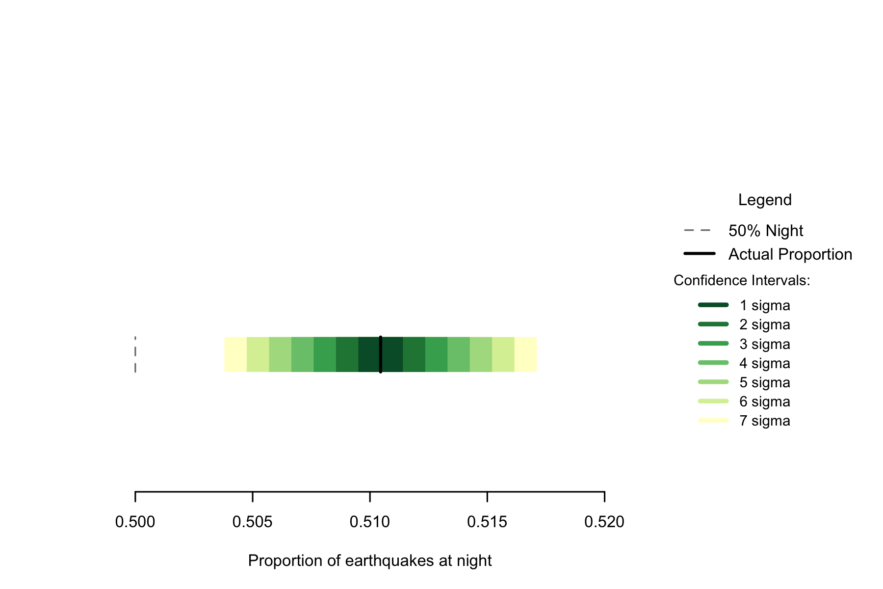
Figure 7.1: Proportion of earthquakes at night: U.S.A. n=278458
While the proportion is not as high as New Zealand’s, the greater number of earthquakes means that the confidence intervals are smaller, so there is more certainty that the rate of night earthquakes is not 50%. Based on New Zealand’s response to earthquakes differing regionally, I would speculate that most of the United States is regions with a low (but still present) response to nighttime.
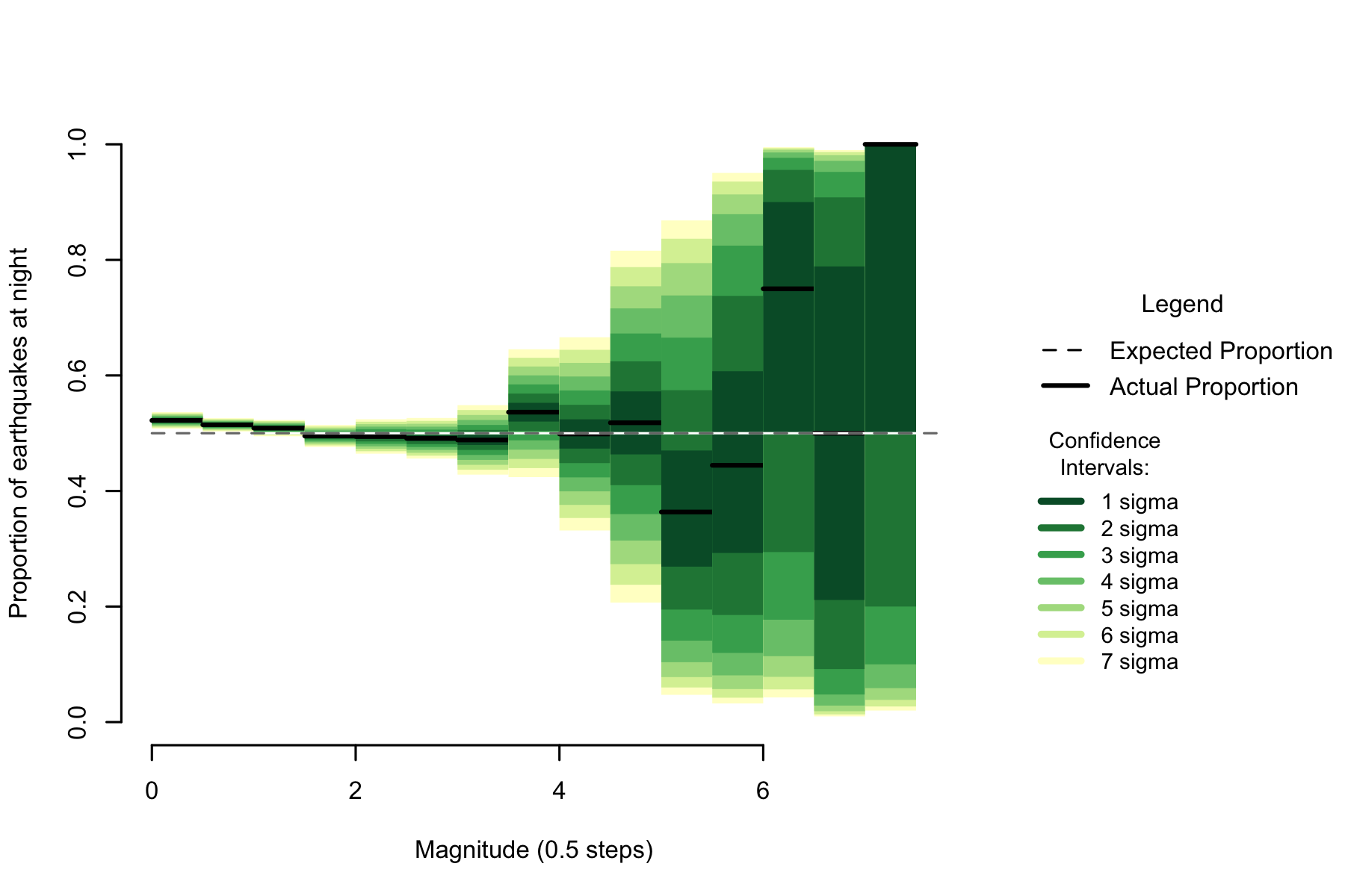
Figure 2.4: Proportion of night earthquakes by magnitude, U.S.A. n=278458
Examining magnitude, there is a similar pattern to New Zealand. Unequivocally high numbers of earthquakes in the low magnitudes falling towards 50% as magnitude increases, then becoming unclear as sample size decreases.
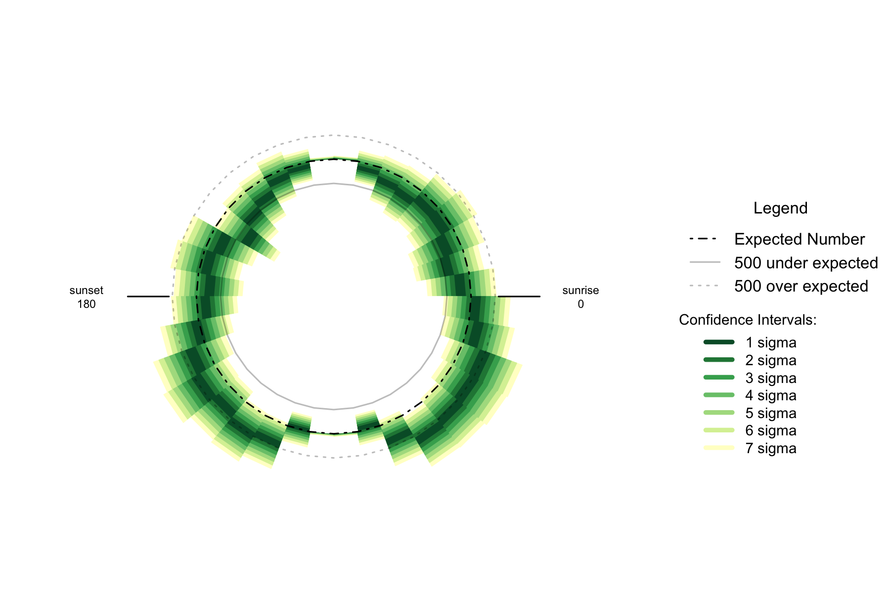
Figure 7.3: Over- and under- supply of earthquakes by angle of the sun (10 degree steps). U.S.A. n=276458
The trend for the number of earthquakes by 10 degree arc of the sun is similar to New Zealand- undersupplies at 30 degrees above the horizon and oversupplies 30-50 degrees below the horizon. The U.S.A. data is skewed slightly compared to New Zealand, as the oversupply is clearly at its greatest when the sun is 30 to 40 degrees below the horizon to the east.
10.1 Formal Statement
Earthquakes in the United States of America show the same pattern as New Zealand, displaying an oversupply of earthquakes at night that is not the result of chance. The magnitude pattern of the oversupply is similar to New Zealand’s pattern, and the pattern with respect to the position of the sun is similar to that of New Zealand.
10.2 Links
1 - USGS: https://earthquake.usgs.gov
10.3 Chapter Code
## ----setup, include=FALSE------------------------------------------------
knitr::opts_chunk$set(echo = FALSE)

## ----c10_001, warnings=FALSE, errors=FALSE, message=FALSE----------------
library(geosphere)
library(lubridate, quietly=TRUE)
library(dplyr)
library(binom)
library(ggplot2)
library(maps)
library(mapdata)
library(parallel)
library(readr)
library(plotrix)
library(tidyr)
library(maptools)
Sys.setenv(TZ = "UTC")


## ----warnings=FALSE, errors=FALSE, message=FALSE-------------------------

if(!dir.exists("../othereqdata")){
  dir.create("../othereqdata")
}
if(!file.exists("../othereqdata/eq_usa_raw.RData")){

begin <- as.POSIXct("2011-09-01 00:00:00", tz="UTC")
end <- as.POSIXct("2016-09-15 00:00:00", tz="UTC")
first <- seq(from=begin, to=end, by="week")
first <- first[1:(length(first)-1)]
second <- first[2:length(first)]
second <- second - seconds(1)
mid_url <- paste("starttime=", format(first, "%Y-%m-%d"), "%20",
                 format(first, "%H:%M:%S"),
                 "&endtime=", format(second, "%Y-%m-%d"), "%20",
                 format(second, "%H:%M:%S"), sep="")
secondlast <- "&maxlatitude=50&minlatitude=24.6&maxlongitude=-65&minlongitude=-125&"
full_url <- paste("https://earthquake.usgs.gov/fdsnws/event/1/query.csv?",
                  mid_url,secondlast,
                  "minmagnitude=0&eventtype=earthquake&orderby=time", sep="")
usgs <- lapply(full_url[1:(length(full_url)-2)],read.csv, stringsAsFactors=FALSE)
equsa <- bind_rows(usgs)
rm(usgs)
equsa$time_UTC <- as.POSIXct(gsub("\\..+","",as.character(equsa$time)),
                             format="%Y-%m-%dT%H:%M:%S", tz="UTC")
eq_national <- equsa %>%
  filter(depth > 0 & mag >= 0 &
           time_UTC >=
           as.POSIXct("2011-09-01T00:00:00", format="%Y-%m-%dT%H:%M:%S", tz="UTC") &
           time_UTC <
           as.POSIXct("2016-09-01T00:00:00", format="%Y-%m-%dT%H:%M:%S", tz="UTC")) %>%
  distinct()  %>% arrange(time_UTC)

rm(equsa)
names(eq_national)[5] <- "magnitude"
save(eq_national, file="../othereqdata/eq_usa_raw.RData")
}

## ------------------------------------------------------------------------

if(!file.exists("../othereqdata/eq_usa_processed.RData")){
load("../othereqdata/eq_usa_raw.RData")
southmost <- min(eq_national$latitude)
westmost <- min(eq_national$longitude)


eq_national <- eq_national %>% filter(
  magnitude > 0, depth > 0) %>% rowwise() %>% mutate(
  eq_gridpoint_y = round(
    distVincentyEllipsoid(c(longitude, southmost),c(longitude,latitude)) /50000,0),
  eq_gridpoint_x = round(
    distVincentyEllipsoid(c(westmost, latitude), c(longitude,latitude)) /50000,0),
  eq_roundedlat = destPoint(
    p=c(longitude, southmost), b=0, d=eq_gridpoint_y*50000)[2],
  eq_roundedlong = destPoint(
    p=c(westmost, eq_roundedlat), b=90, d=eq_gridpoint_x*50000)[1]) %>% ungroup()
# use maptools to calculate solar angles
sun_angles <- solarpos(
  matrix(c(eq_national$longitude, eq_national$latitude), ncol=2), eq_national$time_UTC)
colnames(sun_angles) <- c("eq_compass", "eq_vertical")
eq_national <- cbind(eq_national,sun_angles)
eq_national$eq_is_night <- eq_national$eq_vertical < 0
# calculate 360 degree as well as vertical
eq_national <- eq_national %>%
  mutate(eq_angle_360 = eq_vertical,
         eq_angle_360 = ifelse(eq_compass > 180, 180 - eq_angle_360, eq_angle_360),
         eq_angle_360 = ifelse(eq_vertical < 0 & eq_compass <= 180,
                               360 + eq_angle_360, eq_angle_360),
         eq_angle_by_10 = floor(eq_angle_360 /10) * 10)
save(eq_national, file="../othereqdata/eq_usa_processed.RData")
}

## ------------------------------------------------------------------------
if(!file.exists("../othereqdata/eq_usa_expected.RData")){
load("../othereqdata/eq_usa_processed.RData")

lat_range <- unique(eq_national$eq_roundedlat)
long_med <- median(eq_national$eq_roundedlong)

# 1 minute intervals for a full solar year
time1 <- ymd_hms("2015-01-01 00:00:00")
time2 <- ymd_hms("2015-12-31 23:59:00")
time_sq <- seq.POSIXt(from=time1, to=time2, by="min")


calc_angs <- function(x, longinput, timeinput){
  library(dplyr)
  sun_angles <- maptools::solarpos(matrix(c(longinput, x), ncol=2), timeinput)
  colnames(sun_angles) <- c("eq_compass", "eq_vertical")
# calculate 360 degree as well as vertical
site_summary <- as.data.frame(sun_angles) %>%
  mutate(eq_angle_360 = eq_vertical,
         eq_angle_360 = ifelse(eq_compass > 180, 180 - eq_angle_360, eq_angle_360),
         eq_angle_360 = ifelse(
           eq_vertical < 0 & eq_compass <= 180, 360 + eq_angle_360, eq_angle_360),
         eq_angle_by_10 = floor(eq_angle_360 /10) * 10) %>%
  group_by(eq_angle_by_10) %>% summarise(total= n())
  site_summary$lat <- x
  return(site_summary)
}
###
# Calculate the number of cores
no_cores <- detectCores() - 1
# Initiate cluster
cl <- makeCluster(no_cores)
clusterExport(cl, varlist=c("lat_range", "long_med", "time_sq", "calc_angs"))
list_angs <- parLapply(cl, lat_range,
                         function(x){
                           calc_angs(x=x, longinput=long_med, timeinput=time_sq)})
stopCluster(cl)
###
library(tidyr)
anglong <- bind_rows(list_angs)
angwide <- spread(anglong, key=eq_angle_by_10,value=total)
rm(anglong, list_angs, time_sq)
save(angwide, file="../othereqdata/eq_usa_expected.RData")
}

## ------------------------------------------------------------------------
load("../othereqdata/eq_usa_processed.RData")
load("../othereqdata/eq_usa_expected.RData")
eq_night = sum(eq_national$eq_is_night)
eq_total = nrow(eq_national)
 bands <- rev(c('#ffffcc','#d9f0a3','#addd8e','#78c679','#41ab5d','#238443','#005a32'))
 sigmas <- c(0.682689492137086,
 0.954499736103642,
 0.997300203936740,
 0.999936657516334,
 0.999999426696856,
 0.999999998026825,
 0.999999999997440)
 lbls <- c(
 "1 sigma", "2 sigma",
 "3 sigma", "4 sigma",
 "5 sigma", "6 sigma",
 "7 sigma")
typs <- c(1,1,1,1,1,1,1)
weights <- c(3,3,3,3,3,3,3)
old_par=par()

## ------------------------------------------------------------------------
bt <- binom.test(eq_night ,eq_total, conf.level= .999999999997440)

## ------------------------------------------------------------------------
feature <- c("Earliest (UTC)", "Latest (UTC)",
             "Northernmost", "Southernmost",
             "Westmost", "Eastmost",
             "Percent < Mag 3", "total entries",
             "nighttime quakes")
value <- c(as.character(min(eq_national$time_UTC)),
           as.character(max(eq_national$time_UTC)),
           as.character(max(eq_national$latitude)),
           as.character(min(eq_national$latitude)),
           as.character(min(eq_national$longitude)),
           as.character(max(eq_national$longitude)),
           as.character(round(100*sum(eq_national$magnitude < 3)/eq_total,2)),
           as.character(eq_total),
           as.character(eq_night))
data.frame(feature,value) %>% knitr::kable(caption="Data description")

## ---- fig.cap="Proportion of earthquakes at night: U.S.A. n=278458"------
### making the basic proportion graph
eq_night = sum(eq_national$eq_is_night)
eq_total = nrow(eq_national)
bands <- rev(c('#ffffcc','#d9f0a3','#addd8e','#78c679','#41ab5d','#238443','#005a32'))
sigmas <- c(0.682689492137086,
            0.954499736103642,
            0.997300203936740,
            0.999936657516334,
            0.999999426696856,
            0.999999998026825,
            0.999999999997440)
lbls <- c(
  "1 sigma", "2 sigma",
  "3 sigma", "4 sigma",
  "5 sigma", "6 sigma",
  "7 sigma")
typs <- c(1,1,1,1,1,1,1)
weights <- c(3,3,3,3,3,3,3)
old_par=par()
conf_steps <- function(x, sigmas=sigmas, night=eq_night, total=eq_total){
  ci_lower <- binom.confint(night, total, method=c("wilson"), conf.level = sigmas[x])[1,5]
  ci_upper <- binom.confint(night, total, method=c("wilson"), conf.level = sigmas[x])[1,6]
  ci_data <- data.frame(step = x, ci_lower, ci_upper)
}

ci_spacing <- lapply(7:1, conf_steps, sigmas=sigmas, night=eq_night, total=eq_total)
ci_steps <- bind_rows(ci_spacing)

layout(matrix(c(1,1,1,2), ncol=4))

par(mar=c(5,6,4,2))
plot(c(min(0.5,floor(100*ci_steps[1,2])/100), max(0.5,ceiling(100*ci_steps[1,3])/100)),
       y=c(-3,8), type="n", bty="n", yaxt="n", ylab="",
       xlab="Proportion of earthquakes at night")
a <- a <- apply(ci_steps, 1, function(x){
  polygon(c(x[2], x[3], x[3], x[2]), c(0, 0, 1, 1), col=bands[x[1]], border=NA)})
lines(c(.5,.5), c(0,1), col="#FFFFFF")
lines(c(.5,.5), c(0,1), lty=2, col="#777777")
lines(c(eq_night/eq_total,eq_night/eq_total), c(0,1), lwd=2)

par(mar=c(0,0,0,0))
plot(x=c(0,10), y=c(0,10), type="n", bty="n", axes=FALSE)
legend(0,5.5, legend=lbls, lty=typs, lwd=weights, col=bands, bty="n", xjust=0,
       title="Confidence Intervals:", y.intersp=1.1, cex=0.9)

lbls2=c("50% Night", "Actual Proportion")
typs2=c(2,1)
weights2=c(1,2)
cls2=c("#777777","#000000")
legend(0,7, legend=lbls2, lty=typs2, lwd=weights2, col=cls2, bty="n", xjust=0,
       title="Legend", y.intersp=1.2)


par(mar=old_par$mar)
par(mfrow=c(1,1))


## ---- fig.cap="Proportion of night earthquakes by magnitude, U.S.A. n=278458"----
old_par=par()
grf <- eq_national %>% mutate(floored_mag = floor(magnitude*2)/2) %>%
  group_by(floored_mag) %>% summarise(successes = sum(eq_is_night), trials=n())

poly_conf_int <- function(success, trials, aa, stepsize, sigma, colr){
  ci <- binom.confint(success, trials, method=c("wilson"), conf.level = sigma)
  lower <- ci[1,5]
  upper <- ci[1,6]
  a <- polygon(x=c(aa,aa+stepsize,aa+stepsize,aa), y=c(upper,upper,lower,lower),
               col=colr, border=NA)
}


plot7sig <- function(success, trials, aa, stepsize){
  library(binom)
  #bands <- c('#ffffb2','#fed976','#feb24c','#fd8d3c','#fc4e2a','#e31a1c','#b10026')
  bands <- rev(c('#ffffcc','#d9f0a3','#addd8e','#78c679','#41ab5d','#238443','#005a32'))
  sigmas <- c(0.682689492137086,
              0.954499736103642,
              0.997300203936740,
              0.999936657516334,
              0.999999426696856,
              0.999999998026825,
              0.999999999997440)
  sapply(7:1, function(x){
    poly_conf_int(success, trials, aa, stepsize, sigmas[x], bands[x])})
  a <- lines(c(aa, aa + stepsize), c(success/trials, success/trials), lwd=2)
}


lbls <- c(
  "1 sigma", "2 sigma",
  "3 sigma", "4 sigma",
  "5 sigma", "6 sigma",
  "7 sigma")
typs <- c(1,1,1,1,1,1,1)
weights <- c(3,3,3,3,3,3,3)
clrs <- rev(c('#ffffcc','#d9f0a3','#addd8e','#78c679','#41ab5d','#238443','#005a32'))
#clrs <- c('#ffffb2','#fed976','#feb24c','#fd8d3c','#fc4e2a','#e31a1c','#b10026')

layout(matrix(c(1,1,1,2), ncol=4))
plot(x=c(0,max(grf$floored_mag)+0.5), y=c(0,1), type="n", bty="n",
     xlab="Magnitude (0.5 steps)", ylab="Proportion of earthquakes at night")
a <- apply(grf,1,function(x){plot7sig(x[2],x[3],x[1],0.5)})
lines(c(0,10), c(.5,.5), col="#FFFFFF")
lines(c(0,10), c(.5,.5), lty=2, col="#777777")

par(mar=c(0,0,0,0))
plot(x=c(0,10), y=c(0,10), type="n", bty="n", axes=FALSE)
legend(0,5, legend=lbls, lty=typs, lwd=weights, col=clrs, bty="n", xjust=0,
       title="Confidence
Intervals:", cex=0.9)
lbls=c("Expected Proportion", "Actual Proportion")
typs=c(2,1)
weights=c(1,2)
legend(0,7, legend=lbls, lty=typs, lwd=weights, bty="n", xjust=0,
       title="Legend", y.intersp=1.2)


par(mar=old_par$mar)
par(mfrow=c(1,1))


## ------------------------------------------------------------------------
by_angle <- eq_national %>%
  group_by(eq_angle_by_10) %>% summarise(total= n()) %>%
  mutate(daynight=ifelse(eq_angle_by_10 < 180, "day", "night"))

merged <- merge(eq_national, angwide, by.x="eq_roundedlat", by.y="lat")
agg_expected <- merged %>% select(`0`:`350`) %>% colSums(na.rm=TRUE)
expected_prop <- agg_expected / sum(agg_expected)
expected <- data.frame(eq_angle_by_10 = as.numeric(names(expected_prop)),
                       expected_prop = as.numeric(expected_prop))
expected$expected_number = expected_prop * eq_total
act_exp <- merge(expected, by_angle, by="eq_angle_by_10", all.x=TRUE)

act_exp$total[is.na(act_exp$total)] <- 0
act_exp$daynight <- NULL
act_exp$act_prop <- act_exp$total / sum(act_exp$total)


ci_brackets <- act_exp %>% ungroup() %>% mutate(grand_total=sum(total)) %>%
  rowwise() %>% mutate(
    ci_lower_7 = binom.confint(total, grand_total, method=c("wilson"),
                               conf.level = sigmas[7])[1,5] * grand_total,
    ci_upper_7 = binom.confint(total, grand_total, method=c("wilson"),
                               conf.level = sigmas[7])[1,6] * grand_total,
    ci_lower_6 = binom.confint(total, grand_total, method=c("wilson"),
                               conf.level = sigmas[6])[1,5] * grand_total,
    ci_upper_6 = binom.confint(total, grand_total, method=c("wilson"),
                               conf.level = sigmas[6])[1,6] * grand_total,
    ci_lower_5 = binom.confint(total, grand_total, method=c("wilson"),
                               conf.level = sigmas[5])[1,5] * grand_total,
    ci_upper_5 = binom.confint(total, grand_total, method=c("wilson"),
                               conf.level = sigmas[5])[1,6] * grand_total,
    ci_lower_4 = binom.confint(total, grand_total, method=c("wilson"),
                               conf.level = sigmas[4])[1,5] * grand_total,
    ci_upper_4 = binom.confint(total, grand_total, method=c("wilson"),
                               conf.level = sigmas[4])[1,6] * grand_total,
    ci_lower_3 = binom.confint(total, grand_total, method=c("wilson"),
                               conf.level = sigmas[3])[1,5] * grand_total,
    ci_upper_3 = binom.confint(total, grand_total, method=c("wilson"),
                               conf.level = sigmas[3])[1,6] * grand_total,
    ci_lower_2 = binom.confint(total, grand_total, method=c("wilson"),
                               conf.level = sigmas[2])[1,5] * grand_total,
    ci_upper_2 = binom.confint(total, grand_total, method=c("wilson"),
                               conf.level = sigmas[2])[1,6] * grand_total,
    ci_lower_1 = binom.confint(total, grand_total, method=c("wilson"),
                               conf.level = sigmas[1])[1,5] * grand_total,
    ci_upper_1 = binom.confint(total, grand_total, method=c("wilson"),
                               conf.level = sigmas[1])[1,6] * grand_total)

norm_ci <- ci_brackets

for (i in c(4,7:20)){
norm_ci[,i] <- ci_brackets[,i] - ci_brackets[,3]
}
circlesize=500

## ---- fig.cap="Over- and under- supply of earthquakes by angle of the sun
## (10 degree steps). U.S.A. n=276458"----
norm_ci$border = 2
# need to double entries with a displacement of 10
# to make each side of the item on the graph
norm_ci2 <- norm_ci
norm_ci2$eq_angle_by_10 <- norm_ci2$eq_angle_by_10  + 10
norm_ci2$border = 1
graphdata <-   bind_rows(norm_ci,norm_ci2) %>% arrange(eq_angle_by_10,border)

#### plot graph
bands <- rev(c('#ffffcc','#d9f0a3','#addd8e','#78c679','#41ab5d','#238443','#005a32'))
old_par=par()
layout(matrix(c(1,1,1,2), ncol=4))

# overall limits
limits=2 * max(abs(c(graphdata$ci_lower_7, graphdata$ci_upper_7)))
# plot upper confidence 7 interval using plotrix
polar.plot(graphdata$ci_upper_7, polar.pos=graphdata$eq_angle_by_10,
           radial.lim=c(-1*limits,limits),
           labels = "", main=NULL,lwd=0.5, rp.type="p",
           show.grid.labels=FALSE, show.grid=FALSE, mar=c(0,0,0,0),
           grid.col=bands[7], line.col=bands[7], poly.col=bands[7])
# plot upper 6 confidence interval
plot_ci_round <- function(upper_bound,x){
  polar.plot(upper_bound, polar.pos=graphdata$eq_angle_by_10, add=TRUE,
             radial.lim=c(-1*limits,limits),
             line.col=bands[x], lwd=0.5, rp.type="p", poly.col=bands[x])
}
plot_ci_round(graphdata$ci_upper_6, 6)
plot_ci_round(graphdata$ci_upper_5, 5)
plot_ci_round(graphdata$ci_upper_4, 4)
plot_ci_round(graphdata$ci_upper_3, 3)
plot_ci_round(graphdata$ci_upper_2, 2)
plot_ci_round(graphdata$ci_upper_1, 1)
plot_ci_round(graphdata$ci_lower_1, 2)
plot_ci_round(graphdata$ci_lower_2, 3)
plot_ci_round(graphdata$ci_lower_3, 4)
plot_ci_round(graphdata$ci_lower_4, 5)
plot_ci_round(graphdata$ci_lower_5, 6)
plot_ci_round(graphdata$ci_lower_6, 7)
polar.plot(graphdata$ci_lower_7, polar.pos=graphdata$eq_angle_by_10,
           add=TRUE, radial.lim=c(-1*limits,limits),
           line.col="white", lwd=0.5, rp.type="p", poly.col="white")

# plot expected guide line
polar.plot(rep(0,nrow(graphdata)), polar.pos=graphdata$eq_angle_by_10, add=TRUE,
           radial.lim=c(-1*limits,limits),
           rp.type="p", lty=4)
# plot 500 less than expected guide line
polar.plot(rep(-1 * circlesize,nrow(graphdata)), polar.pos=graphdata$eq_angle_by_10,
           add=TRUE,radial.lim=c(-1*limits,limits),
           rp.type="p", lty=1, line.col="#00000044")
# plot 500 more than expected guide line
polar.plot(rep(circlesize,nrow(graphdata)), polar.pos=graphdata$eq_angle_by_10,
           add=TRUE,radial.lim=c(-1*limits,limits),
           rp.type="p", lty=3, line.col="#00000044")

lines(c(-1.5,-1.2)*limits, c(0,0))
lines(c(1.5,1.2)*limits, c(0,0))
text(-1.8*limits,0, label="sunset
180", cex=0.7)
text(1.8*limits,0, label="sunrise
0", cex=0.7)


par(mar=c(0,0,0,0))
plot(x=c(0,10), y=c(0,10), type="n", bty="n", axes=FALSE, xlab="")
lbls <- c(
  "1 sigma", "2 sigma",
  "3 sigma", "4 sigma",
  "5 sigma", "6 sigma",
  "7 sigma")
typs <- c(1,1,1,1,1,1,1)
weights <- c(3,3,3,3,3,3,3)
clrs <- rev(c('#ffffcc','#d9f0a3','#addd8e','#78c679','#41ab5d','#238443','#005a32'))
legend(0,4.5, legend=lbls, lty=typs, lwd=weights, col=clrs, bty="n", xjust=0,
       title="Confidence Intervals:", cex=0.9)

lbls2=c("Expected Number", paste(circlesize,"under expected"),
        paste(circlesize,"over expected"))
typs2=c(4,1,3)
weights2=c(1,1,1)
clrs2=c("#000000","#00000044","#00000044")
legend(0,10, legend=lbls2, lty=typs2, lwd=weights2, bty="n", xjust=0,
       title="Legend", y.intersp=1.2, col=clrs2)


par(mar=old_par$mar)
par(mfrow=c(1,1))