Chapter 7 It is not the moon
The question “could it be the moon” tends to come from people who have heard a lot of commentary about the moon and earthquakes. But the moon’s daily rotation around the earth is not the same as the sun’s rotation, taking on average 24 hours and 50 minutes for full rotational cycle. This extended period compared to the solar day means that, over longs periods of time, the moon is present in the day as much as the moon is present at night. So the effects of the moon are present in the day as much as the night. I have chosen to omit several hundred lines of code demonstrating empirically this is the case, on the grounds that it is not logically possible for it to be otherwise, so the code was a bit of a distraction.
The moon is the principle component of the solid earth tide, the deformation of the globe caused by tidal forces acting on the molten interior of the earth. This gravity-based effect causes displacement of the ground on an approximately 12.5 hour repeating cycle, with typical displacement of the ground around half a metre in that period. Though this is regular geological activity and stress, the pattern of earthquake frequency in no way resembles a 12.5 hour repeating cycle, so this is not solely the solid earth tide.
Up until now, I have been describing day and night as general categories, and asserting the moon does not make logical sense. Rather than looking at earthquakes in a general night/ day distinction we can focus on more specific 10 degree arcs of the sun.
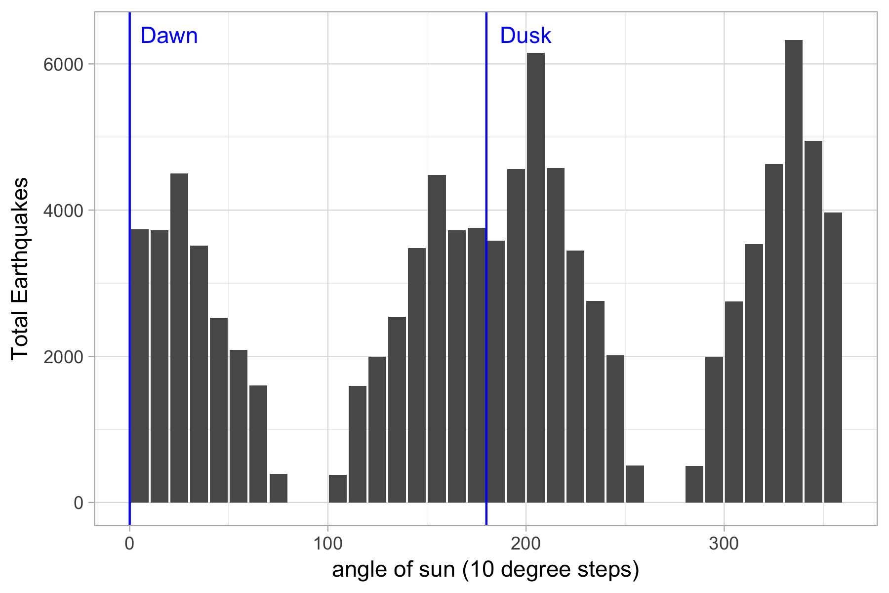
Figure 2.1: Number of earthquakes by 10 degree arcs of angle of the sun at time of earthquake
By eye, there is a difference of thousands in the time a little either side of dawn and dusk with little difference (or earthquakes) at other times. As one form of day/ night comparison, I can compare each group with that 180 degrees apart.
| day angle | day_n | night_n | difference |
|---|---|---|---|
| 0 | 3735 | 3580 | -155 |
| 10 | 3723 | 4565 | 842 |
| 20 | 4501 | 6150 | 1649 |
| 30 | 3512 | 4574 | 1062 |
| 40 | 2529 | 3449 | 920 |
| 50 | 2091 | 2760 | 669 |
| 60 | 1599 | 2014 | 415 |
| 70 | 393 | 504 | 111 |
| 100 | 376 | 497 | 121 |
| 110 | 1595 | 1993 | 398 |
| 120 | 1993 | 2749 | 756 |
| 130 | 2542 | 3535 | 993 |
| 140 | 3481 | 4630 | 1149 |
| 150 | 4479 | 6329 | 1850 |
| 160 | 3724 | 4947 | 1223 |
| 170 | 3760 | 3970 | 210 |
Assuming it is valid to compare day against night with a 180 degree rotation (which I don’t actually know, but is a handy assumption), there does seem to more earthquakes at night than the day when the sun is in the early or late part of the orbit relative to the horizon rather than in the middle of the day or night.
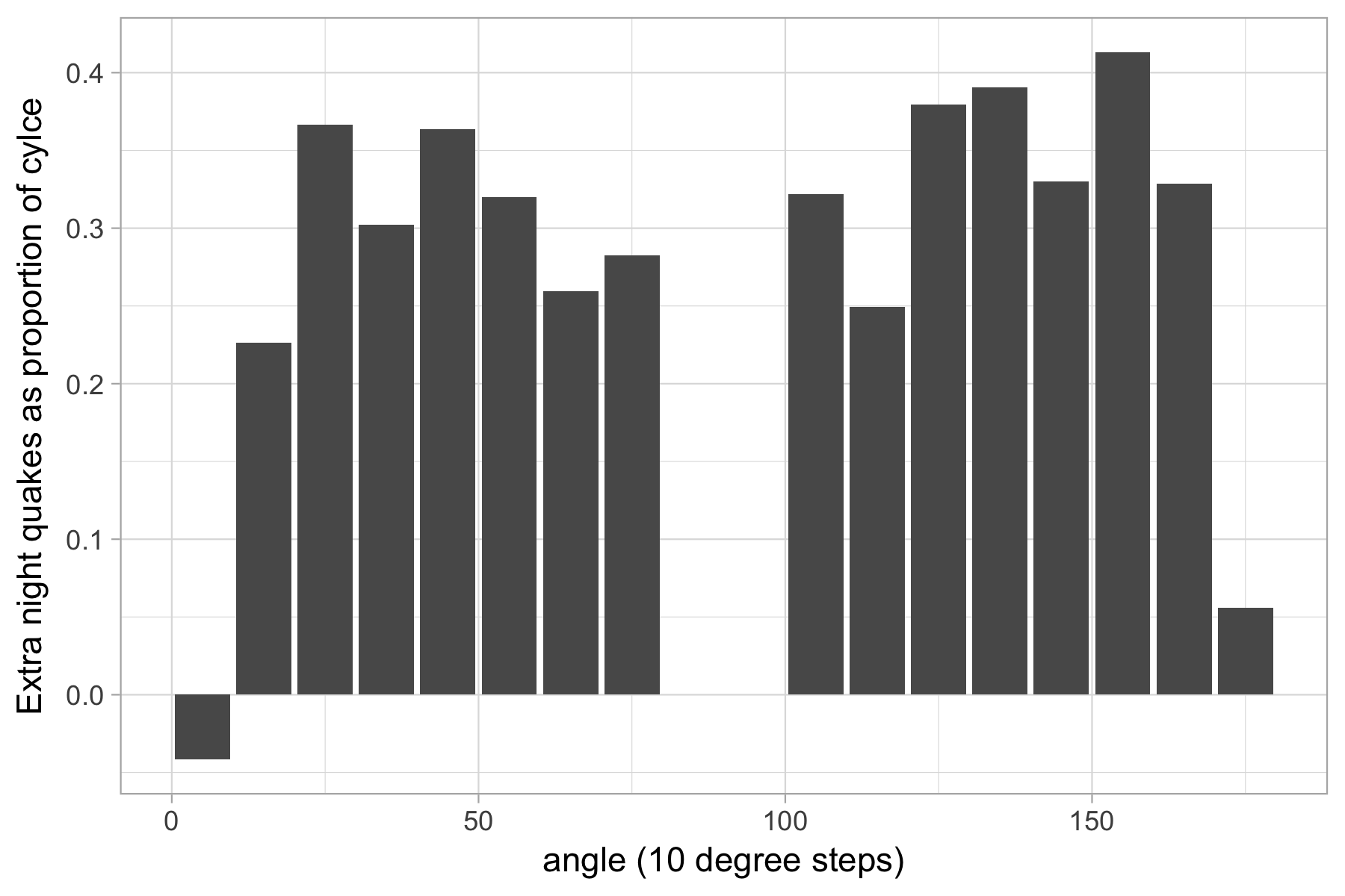
Figure 2.2: excess of night compared to 180 different sun position, as proportion of number of earthquakes in the day position
But I haven’t established that rotating day is a reasonable basis for comparison, it is just useful.
A better approach is to figure out how many earthquakes are expected in each arc of the sun, and how many actually occurred. I can do this by calculating what angle the sun was at for a solar year for each earthquake site, and adding up how many occurrences at each angle. This gives the percentage of time the sun was in each arc of the sky. If the number of earthquakes (as a percentage of the total earthquakes) is greater than the percentage of time for the earthquakes to occur (in that arc of the sun) then there are more earthquakes than expected.
While the sun arcs for each individual site can be calculated, it takes many hours and the calculations get longer as the data grows. I can dramatically speed up the calculations by making a few simplifying assumptions
Given the size of the planet, the sun angles are very similar for sites with fifty kilometres. So rather than calculating the sun angles for each site, I can calculate the sun angles for the 50 km square grid points.
While potential sun angles change with latitude, over the long term longitude is displaced slightly in time but will add to the same total, so I only need to calculate the latitude steps.
I checked this, and found it gave me the same overall answers as doing all the individual calculations, so I am taking the gridded approach here. I am also using the parallel library in R to speed up the grid calculations over several cores on my computer. Your computer may not be the same in this respect.
By combining the gridded counts together with the original data I can get an observed versus expected numbers for each arc. There is a choice of ways of thinking about the problem here. We can think of the differences shown in absolute terms where there are a certain number of earthquakes above or below the expected amount, or in relative terms where there are more or less earthquakes in proportion to the number of earthquakes that happen.
7.1 Absolute difference
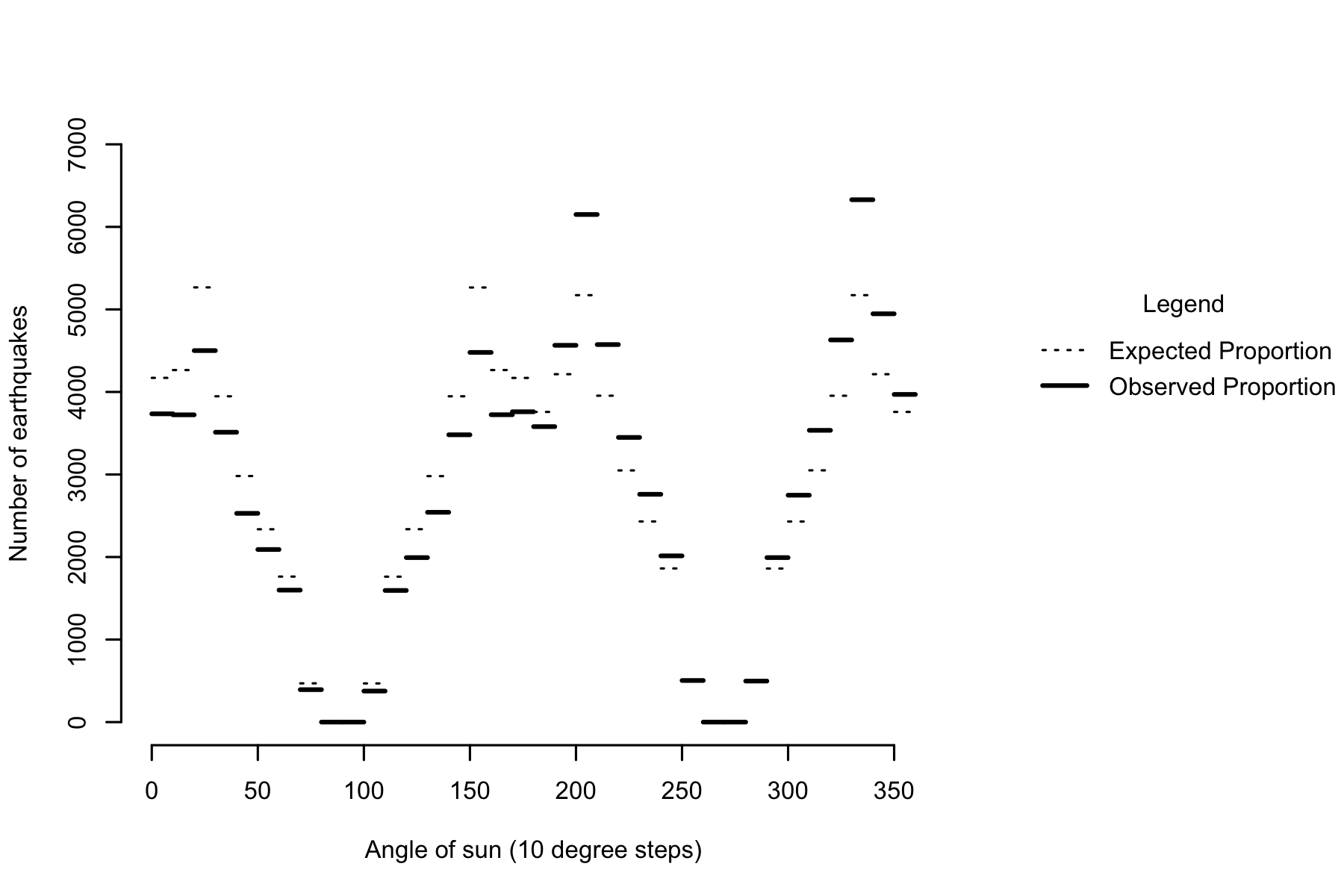
Figure 7.1: Comparison of expected to observed earthquakes by angle of the sun
From comparing expected with observed, it is the case that there are both fewer earthquakes than expected during the day and more earthquakes than expected at night. To get a sense of how reliable these differences are, I can add confidence intervals to the observed data, to give a sense of how far away we might expect the “true” expected proportion to be.
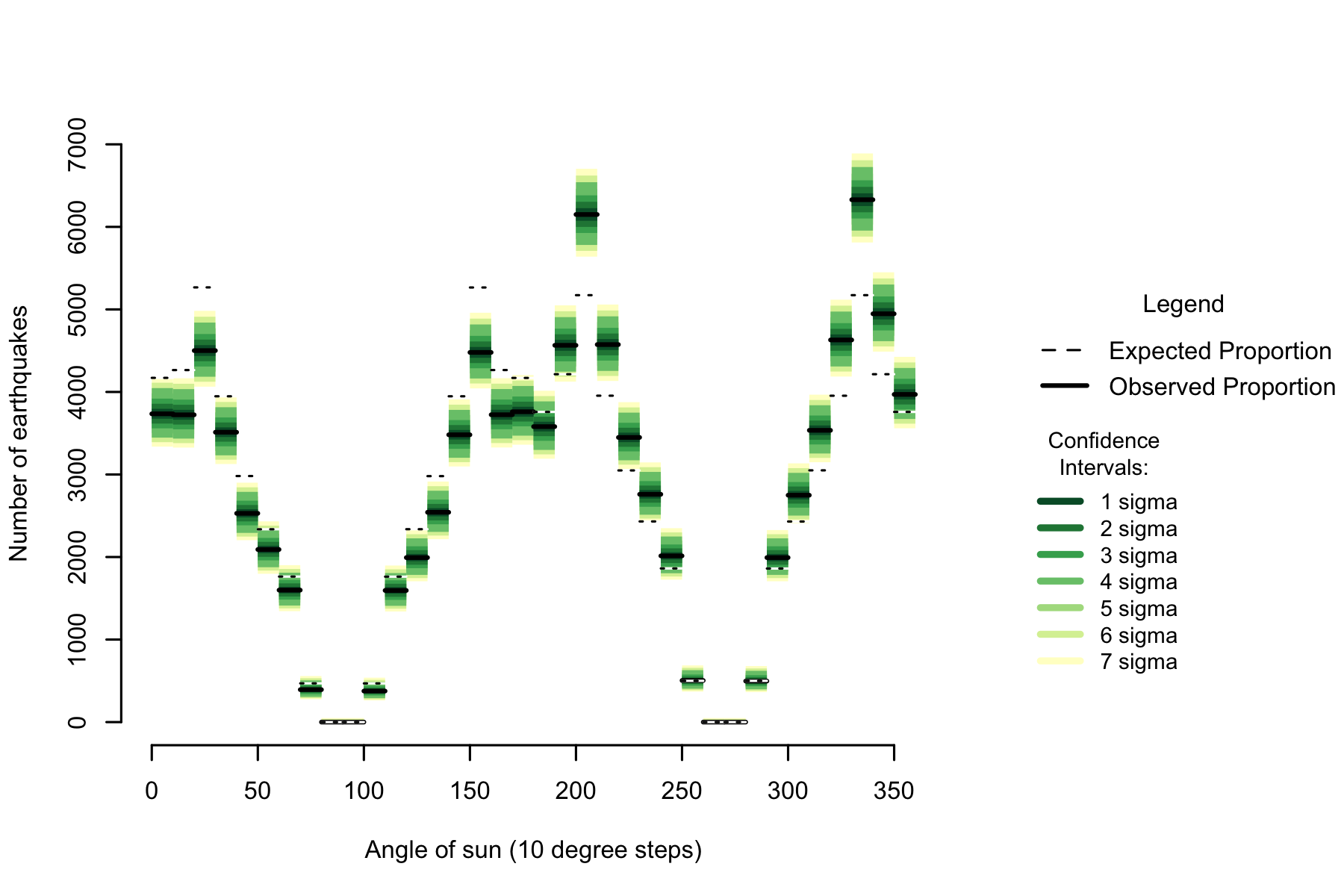
Figure 7.2: Comparison of expected to observed (with uncertainty) earthquakes by angle of the sun
Compared against an expected value based on all earthquakes and all available time, earthquakes are unusually low during the day and night. Except for around dawn and dusk (when it crosses from day to night) and near the middle of the night when there are very few earthquakes. This difference in actual versus expected earthquakes can be better seen by making a graph based on how far from the expected amount is each 10 degree sun arc.
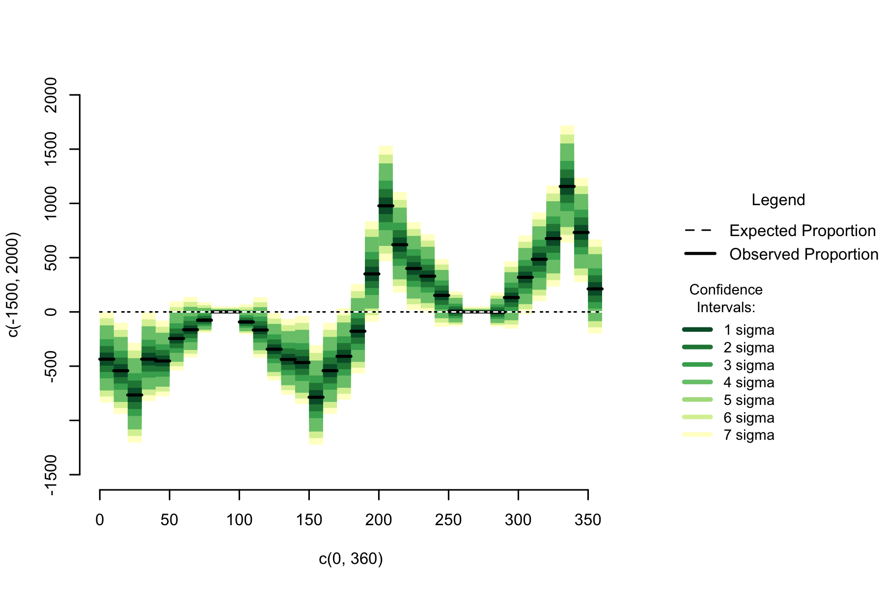
Figure 7.3: Difference of observed earthquake numbers from expected by 10 degree sun arc
On the graph the locations around 30 degrees away from the horizon seem to be particularly unusual points. However, the orbit of the sun is not linear, it is circular(-ish)
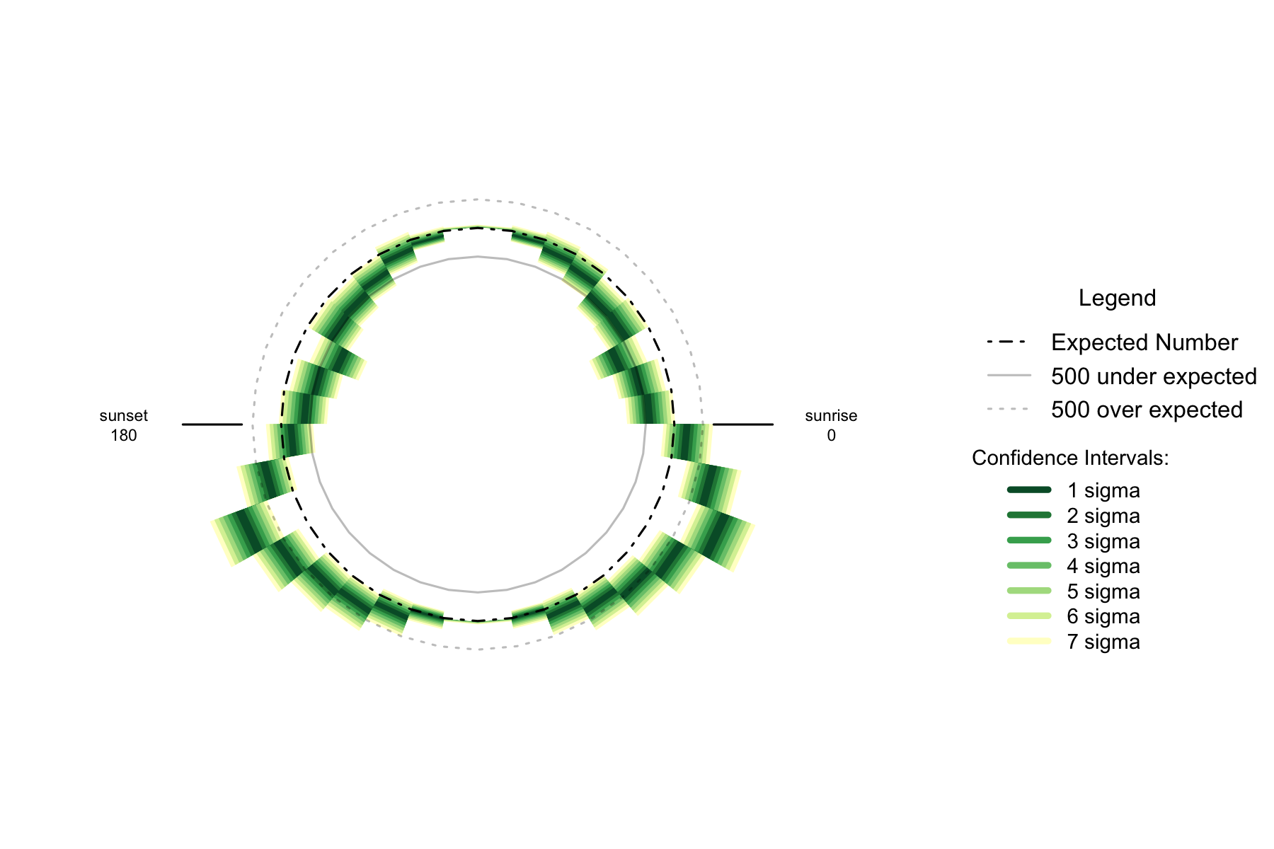
Figure 2.5: Oversupply of earthquakes compared to expected number in suns orbit (10 degree steps)
While the areas 30 degrees above the horizon stand out as a little out of line with the overall pattern in their region, the overall shape is being most influenced by an overabundance of earthquakes focused on thirty degrees below the horizon.
This is not a lunar pattern. Even taking the solar component of the solid earth tide, it is not the same pattern. The solid earth tide contracts the local ground when the gravitational sources are near the horizon, and expands the earth when the gravitational sources are a midnight or midday.
7.2 Relative
A second way of looking at the difference of expected to actual earthquakes is in the relationships between rising counts of earthquakes.
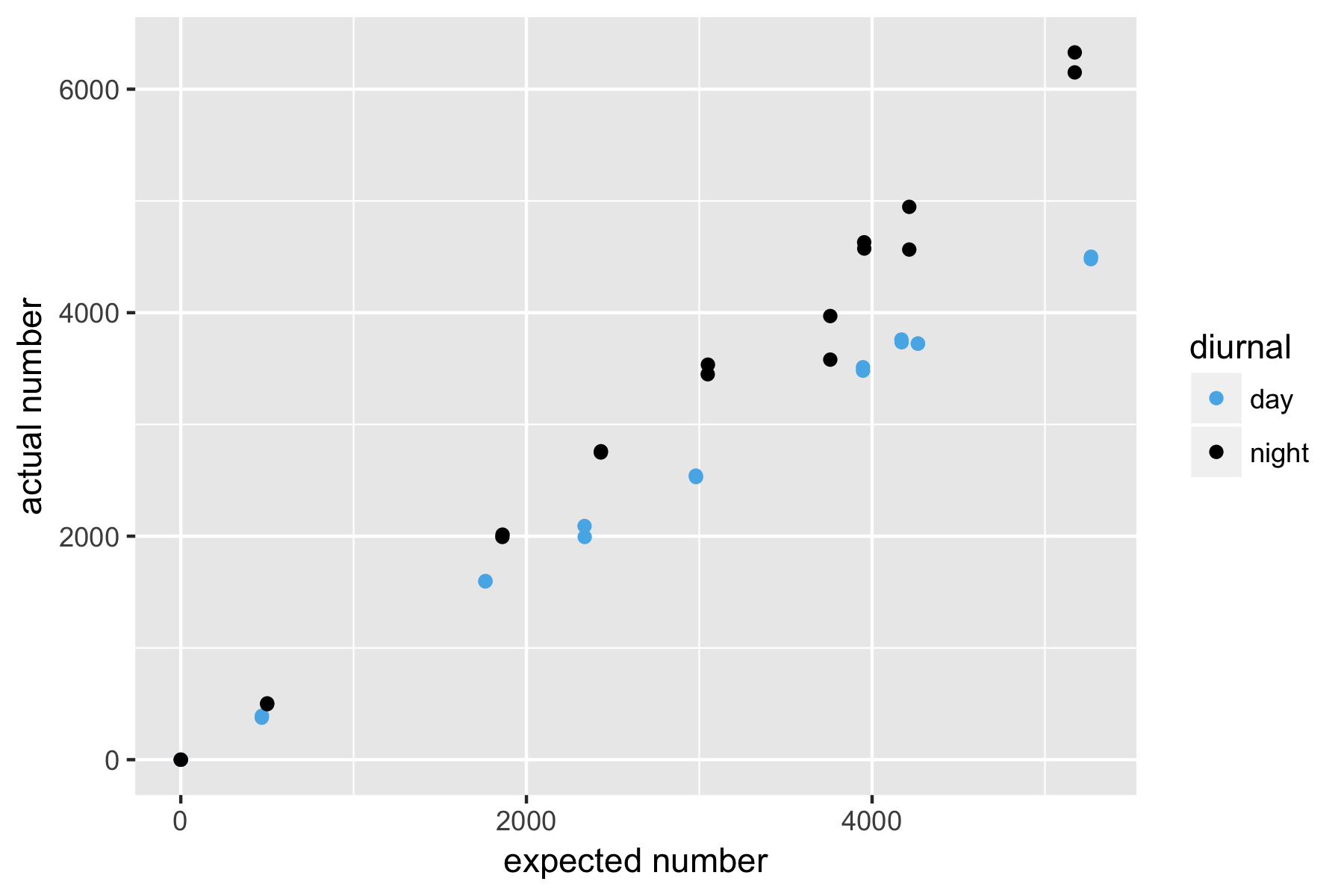
Figure 7.4: Actual vs expected number of earthquakes by diurnal cycle
The points do seem to be forming two lines that diverge as the number of earthquakes increase. For this reason, I think it makes sense to calculate a different line of best fit for both night and day.
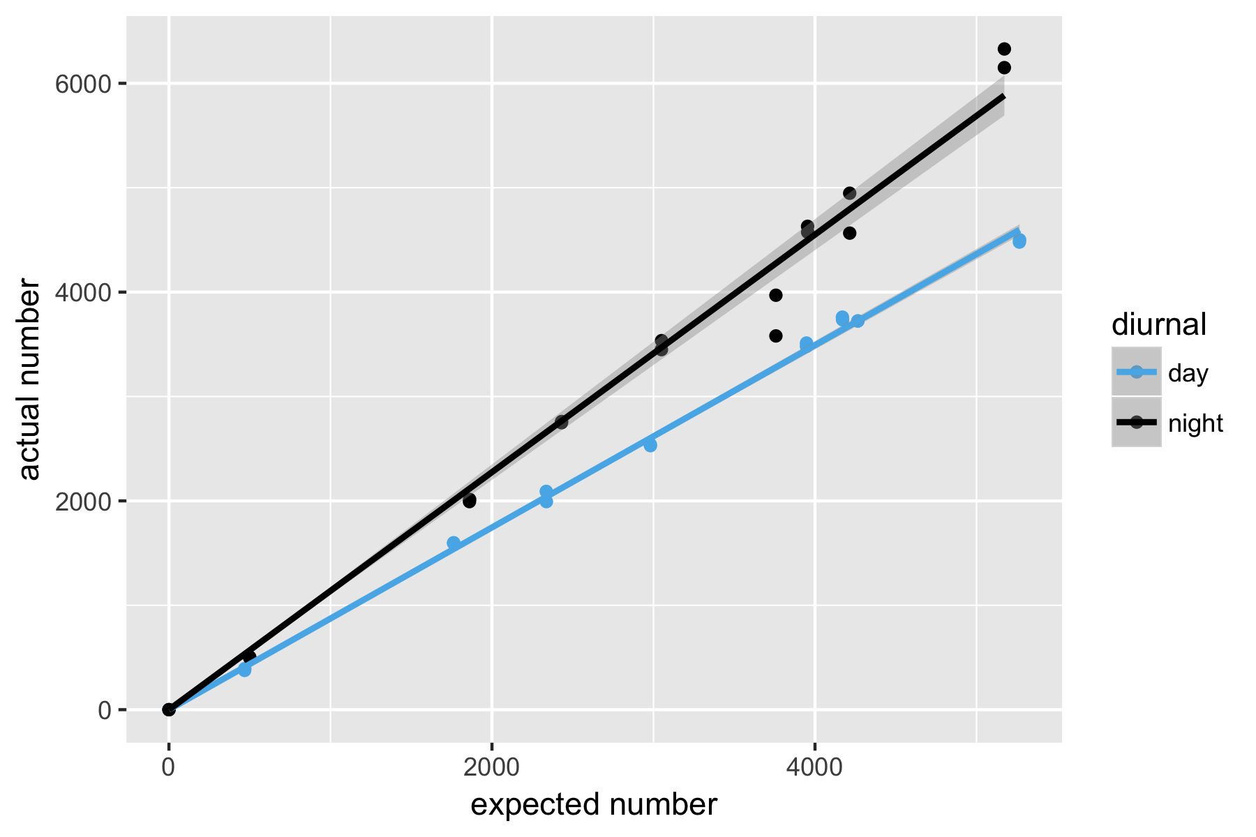
Figure 7.5: Best fit lines of actual vs expected number of earthquakes
Starting from zero, as with zero opportunities for earthquakes I am assuming there will be zero earthquakes, there are 0.872751 earthquakes in the day for “expected” quake. The Adjusted R-squared value of 0.9995 means that this line is an almost perfect fit to the data. For the night earthquakes there are 1.13761 earthquakes for each expected quake. The Adjusted R-squared value of 0.9959 is a line not quite as perfectly fitting as the day, but still very perfect.
By way of cross-checking the night earthquakes were 1.303476 as common as day ones, which accords with the overall values of night versus day. The good fit of the lines suggests that this is a good model for the data.
After fitting a linear model like this, it is standard practice to check the residuals- to see if there is a pattern to the amount of variation to the line of best fit.
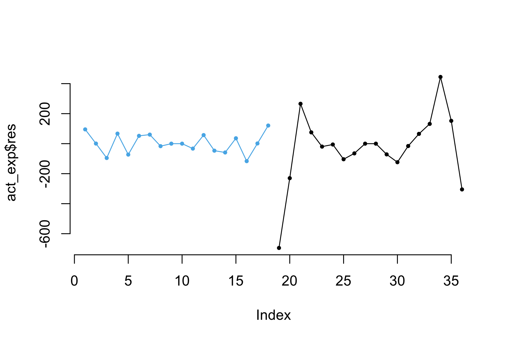
Figure 7.6: Variation in raw residuals
Viewed in degree order from 0 to 360 degrees, there are peaks in the early hours of the night.
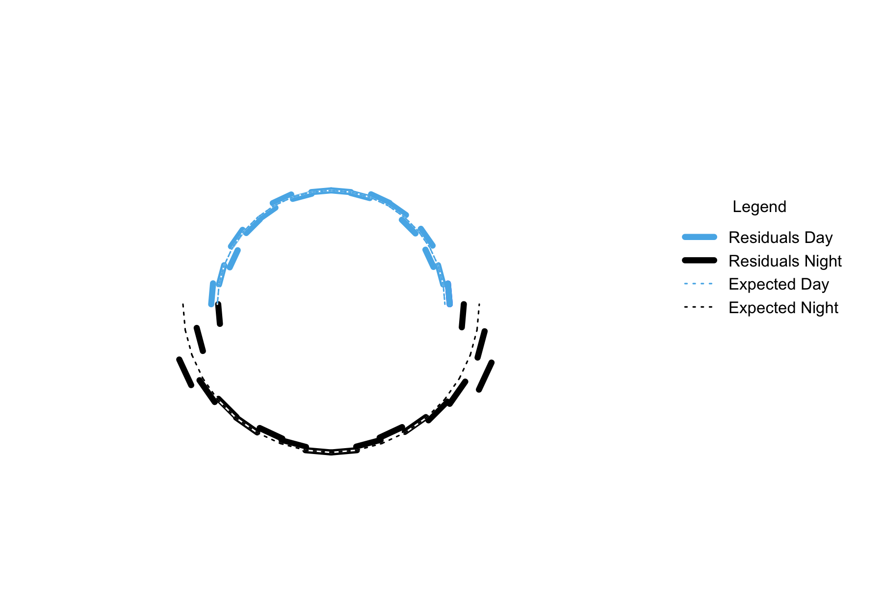
Figure 7.7: Rotational variation in residuals. The nightly residuals have been displaced by the mean difference between day and night, to reflect the different between the two lines
The over pattern is of unusual numbers of earthquakes peaking when the sun is around 30 degrees below the horizon, with daytime showing no unusual patterns.This result is broadly similar to that of the absolute value proportions for each arc. The pattern is reflectively symmetrical around midnight or midday based on unusual early/late night peaks.
The irregular residuals occurring at night, with the day being completely regular, is interesting by itself. It suggests that the unusual earthquake behaviour is nightly rather than daily.
This symmetry does not at all match the lunar component of the solid earth tide, nor does it match the much weaker solar component. The earth’s crust is contracted when the source of gravity is near the horizon (for the sun, dusk and dawn), and expanded when the source of gravity is directly above or below (for the sun, midnight and midday). A peak only at night, about halfway between the maximum solid earth tide effects does not match this pattern.
But the solid earth tide is affecting the pattern of earthquakes. Categorising time periods into night and day for the sun and if the earth’s crust is in a contracted or expanded state from the solid earth tide, if the events were independent there should be a similar number of earthquakes in each category.
| solidearth | diurnal | total |
|---|---|---|
| contracted | day | 25026 |
| contracted | night | 35951 |
| expanded | day | 19007 |
| expanded | night | 20295 |
Because the earth is not a perfect sphere, in New Zealand the crust is in a contracted state most of the time relative to the baseline of the hypothetical sphere, so the number of earthquakes when the solid earth is contracted is not expected to be the same as when it is expanded. However, the earth is contracted (and expanded) for the same amount of time in both night and day. The big difference in the number of earthquakes between night and day when the earth is contracted, compared to the small difference in the number of earthquakes between night and day when the earth is expanded, suggests that the solid earth tide does have some effect on the process, even though the tide is not the primary cause.
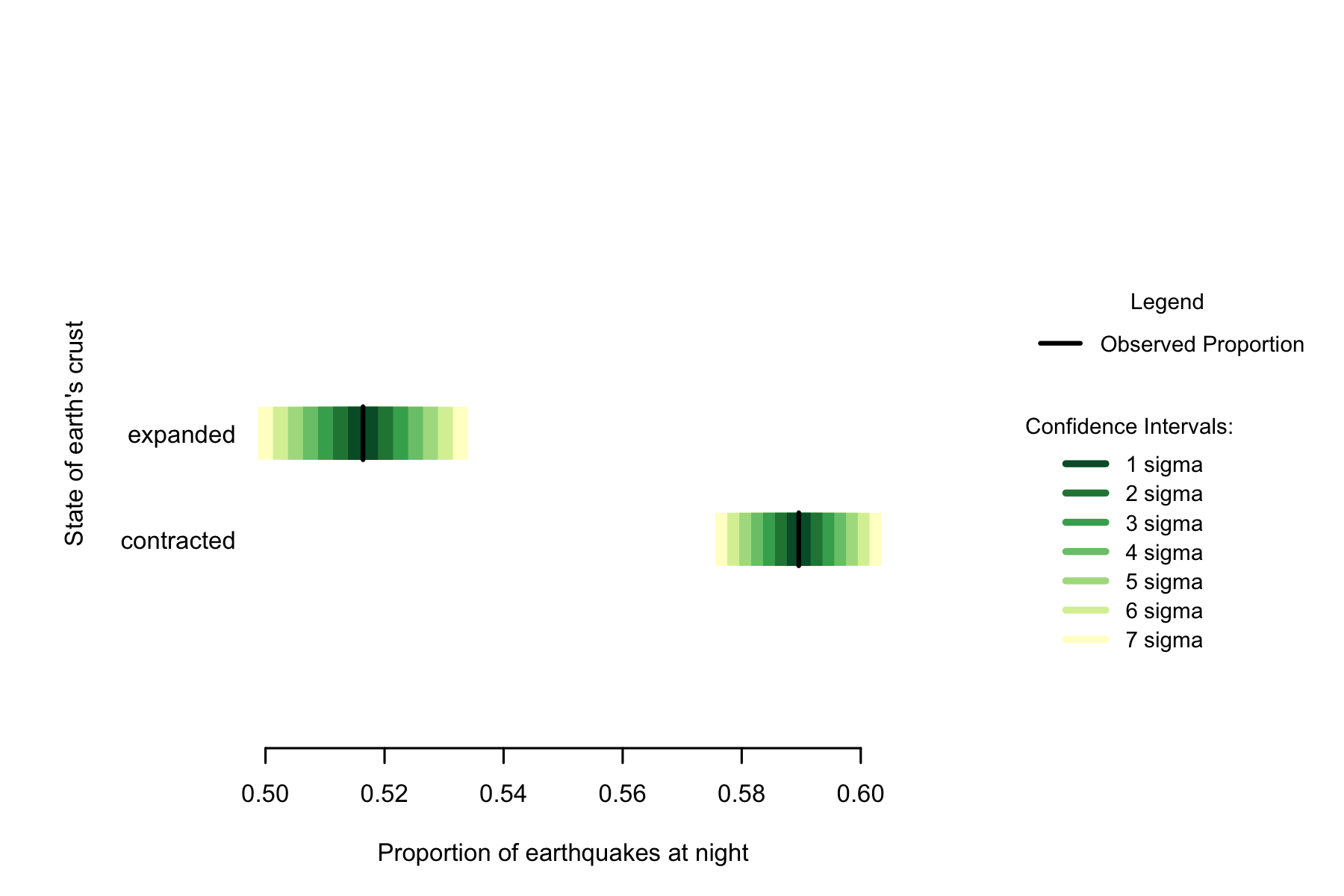
Figure 7.8: Solid earth tide and proportion of earthquakes at night
This monograph is not about the solid earth tide effects, so I am only noting that the solid earth tide has a significant effect on the pattern of earthquakes. To my knowledge no-one has found this effect before.
7.3 Formal Statement
The diurnal pattern of earthquakes is inconsistent with the moon being the direct cause. However, the solid earth tide, of which the moon is the major component, has a significant role in the frequency patterns of earthquakes.
7.5 Chapter Code
## ----setup, include=FALSE------------------------------------------------
knitr::opts_chunk$set(echo = FALSE)
knitr::opts_chunk$set(warnings=FALSE)
knitr::opts_chunk$set(errors=FALSE)
knitr::opts_chunk$set(message=FALSE)
knitr::opts_chunk$set(dpi = 150)
knitr::opts_chunk$set(fig.width =  6)
knitr::opts_chunk$set(fig.height =  4)

## ----c002_libraries------------------------------------------------------
Sys.setenv(TZ = "UTC")
library(dplyr)
library(ggplot2)
library(lubridate)
library(maptools)
library(binom)
library(parallel)
library(plotrix)
library(solidearthtide)
library(tidyr)
# Assumes there is eqnz_processed data created in chapter 2
load("eqdata/eqnz_processed.RData")
old_par <- par()

lbls <- c(
 "1 sigma", "2 sigma",
 "3 sigma", "4 sigma",
 "5 sigma", "6 sigma",
 "7 sigma")
typs <- c(1,1,1,1,1,1,1)
weights <- c(3,3,3,3,3,3,3)
clrs <- rev(c('#ffffcc','#d9f0a3','#addd8e','#78c679','#41ab5d','#238443','#005a32'))
circlesize=500


## ----fig.cap=
##"Number of earthquakes by 10 degree arcs of angle of the sun at time of earthquake"----
by_angle <- eqnz %>%
  group_by(eq_angle_by_10) %>% summarise(total= n()) %>%
  mutate(daynight=ifelse(eq_angle_by_10 < 180, "day", "night"))

ggplot(data=by_angle, aes(x=eq_angle_by_10+5, y=total)) +
  geom_bar(stat="identity") +
  xlab("angle of sun (10 degree steps)") + ylab("Total Earthquakes") +
  geom_vline(xintercept = c(0,180), colour="blue") +
  annotate("text", x = 20, y = 6400, label = "Dawn", color="blue") +
  annotate("text", x = 200, y = 6400, label = "Dusk", color="blue") + theme_light()

## ----results="asis"------------------------------------------------------
only180 = by_angle[1:16,]
only180$night = by_angle$total[17:32]
only180$difference = only180$night - only180$total
only180$asprop = only180$difference / only180$total
only180 %>% select(`day angle`=eq_angle_by_10, day_n=total,
                   night_n=night, difference) %>% knitr::kable(
             caption="180 degree comparison of day and night")

## ---- fig.cap="excess of night compared to 180 different sun position, as proportion
## of number of earthquakes in the day position"----
ggplot(data=only180, aes(x=eq_angle_by_10+5, y=asprop)) +
  geom_bar(stat="identity") +
  xlab("angle (10 degree steps)") + ylab("Extra night quakes as proportion of cylce") +
  theme_light()

## ------------------------------------------------------------------------
if (!file.exists("eqdata/eqnz_expected.RData")){
lat_range <- unique(eqnz$eq_roundedlat)
long_med <- median(eqnz$eq_roundedlong)

# 1 minute intervals for a full solar year
time1 <- ymd_hms("2015-01-01 00:00:00")
time2 <- ymd_hms("2015-12-31 23:59:00")
time_sq <- seq.POSIXt(from=time1, to=time2, by="min")


calc_angs <- function(x, longinput, timeinput){
  library(dplyr)
  sun_angles <- maptools::solarpos(matrix(c(longinput, x), ncol=2), timeinput)
  colnames(sun_angles) <- c("eq_compass", "eq_vertical")
# calculate 360 degree as well as vertical
site_summary <- as.data.frame(sun_angles) %>%
  mutate(eq_angle_360 = eq_vertical,
         eq_angle_360 = ifelse(eq_compass > 180, 180 - eq_angle_360, eq_angle_360),
         eq_angle_360 = ifelse(eq_vertical < 0 & eq_compass <= 180,
                               360 + eq_angle_360, eq_angle_360),
         eq_angle_by_10 = floor(eq_angle_360 /10) * 10) %>%
  group_by(eq_angle_by_10) %>% summarise(total= n())
  site_summary$lat <- x
  return(site_summary)
}
###
# Calculate the number of cores
no_cores <- detectCores() - 1
# Initiate cluster
cl <- makeCluster(no_cores)
clusterExport(cl, varlist=c("lat_range", "long_med", "time_sq", "calc_angs"))
list_angs <- parLapply(
  cl, lat_range, function(x){
                           calc_angs(x=x, longinput=long_med, timeinput=time_sq)})
stopCluster(cl)
###
library(tidyr)
anglong <- bind_rows(list_angs)
angwide <- spread(anglong, key=eq_angle_by_10,value=total)
rm(anglong, list_angs, time_sq)
save(angwide, file="eqdata/eqnz_expected.RData")
}
load("eqdata/eqnz_expected.RData")

## ------------------------------------------------------------------------
grand_total <- nrow(eqnz)
merged <- merge(eqnz, angwide, by.x="eq_roundedlat", by.y="lat")
agg_expected <- merged %>% select(`0`:`350`) %>% colSums(na.rm=TRUE)
expected_prop <- agg_expected / sum(agg_expected)
expected <- data.frame(eq_angle_by_10 = as.numeric(names(expected_prop)),
                       expected_prop = as.numeric(expected_prop))
expected$expected_number = expected_prop * grand_total
act_exp <- merge(expected, by_angle, by="eq_angle_by_10", all.x=TRUE)
act_exp$total[is.na(act_exp$total)] <- 0
act_exp$daynight <- NULL
act_exp$act_prop <- act_exp$total / sum(act_exp$total)

## ---- fig.cap="Comparison of expected to observed earthquakes by angle of the sun"----
old_par=par()
layout(matrix(c(1,1,1,2), ncol=4))
plot(c(0,360),c(0,7000), bty="n", type="n",
     ylab="Number of earthquakes", xlab="Angle of sun (10 degree steps)")
a <- apply(act_exp[,c(1,4)], 1, function(x){lines(c(x[1], x[1]+10), c(x[2],x[2]), lwd=2)})
a <- apply(act_exp[,c(1,3)], 1, function(x){lines(c(x[1], x[1]+10), c(x[2],x[2]), lty=3)})

par(mar=c(0,0,0,0))
plot(x=c(0,10), y=c(0,10), type="n", bty="n", axes=FALSE)
lbls=c("Expected Proportion", "Observed Proportion")
typs=c(3,1)
weights=c(1,2)
legend(0,7, legend=lbls, lty=typs, lwd=weights, bty="n",
       xjust=0,
       title="Legend", y.intersp=1.2)


par(mar=old_par$mar)
par(mfrow=c(1,1))


## --------------------------------------------------------------

 sigmas <- c(0.682689492137086,
 0.954499736103642,
 0.997300203936740,
 0.999936657516334,
 0.999999426696856,
 0.999999998026825,
 0.999999999997440)

ci_brackets <- act_exp %>% ungroup() %>% mutate(grand_total=sum(total)) %>%
  rowwise() %>% mutate(
    ci_lower_7 = binom.confint(total, grand_total, method=c("wilson"),
                               conf.level = sigmas[7])[1,5] * grand_total,
    ci_upper_7 = binom.confint(total, grand_total, method=c("wilson"),
                               conf.level = sigmas[7])[1,6] * grand_total,
    ci_lower_6 = binom.confint(total, grand_total, method=c("wilson"),
                               conf.level = sigmas[6])[1,5] * grand_total,
    ci_upper_6 = binom.confint(total, grand_total, method=c("wilson"),
                               conf.level = sigmas[6])[1,6] * grand_total,
    ci_lower_5 = binom.confint(total, grand_total, method=c("wilson"),
                               conf.level = sigmas[5])[1,5] * grand_total,
    ci_upper_5 = binom.confint(total, grand_total, method=c("wilson"),
                               conf.level = sigmas[5])[1,6] * grand_total,
    ci_lower_4 = binom.confint(total, grand_total, method=c("wilson"),
                               conf.level = sigmas[4])[1,5] * grand_total,
    ci_upper_4 = binom.confint(total, grand_total, method=c("wilson"),
                               conf.level = sigmas[4])[1,6] * grand_total,
    ci_lower_3 = binom.confint(total, grand_total, method=c("wilson"),
                               conf.level = sigmas[3])[1,5] * grand_total,
    ci_upper_3 = binom.confint(total, grand_total, method=c("wilson"),
                               conf.level = sigmas[3])[1,6] * grand_total,
    ci_lower_2 = binom.confint(total, grand_total, method=c("wilson"),
                               conf.level = sigmas[2])[1,5] * grand_total,
    ci_upper_2 = binom.confint(total, grand_total, method=c("wilson"),
                               conf.level = sigmas[2])[1,6] * grand_total,
    ci_lower_1 = binom.confint(total, grand_total, method=c("wilson"),
                               conf.level = sigmas[1])[1,5] * grand_total,
    ci_upper_1 = binom.confint(total, grand_total, method=c("wilson"),
                               conf.level = sigmas[1])[1,6] * grand_total)


## ---- fig.cap="Comparison of expected to observed
## (with uncertainty) earthquakes by angle of the sun"----
bands <- rev(c('#ffffcc','#d9f0a3','#addd8e','#78c679','#41ab5d','#238443','#005a32'))
old_par=par()
layout(matrix(c(1,1,1,2), ncol=4))
plot(c(0,360),c(0,7000), bty="n", type="n",
     ylab="Number of earthquakes", xlab="Angle of sun (10 degree steps)")
a <- apply(ci_brackets, 1, function(x){polygon(c(x[1], x[1]+10, x[1]+10, x[1]),
                                               c(x[7],x[7], x[8],x[8]),
                                               col=bands[7], border=NA)})
a <- apply(ci_brackets, 1, function(x){polygon(c(x[1], x[1]+10, x[1]+10, x[1]),
                                               c(x[9],x[9], x[10],x[10]),
                                               col=bands[6], border=NA)})
a <- apply(ci_brackets, 1, function(x){polygon(c(x[1], x[1]+10, x[1]+10, x[1]),
                                               c(x[11],x[11], x[12],x[12]),
                                               col=bands[4], border=NA)})
a <- apply(ci_brackets, 1, function(x){polygon(c(x[1], x[1]+10, x[1]+10, x[1]),
                                               c(x[13],x[13], x[14],x[14]),
                                               col=bands[4], border=NA)})
a <- apply(ci_brackets, 1, function(x){polygon(c(x[1], x[1]+10, x[1]+10, x[1]),
                                               c(x[15],x[15], x[16],x[16]),
                                               col=bands[3], border=NA)})
a <- apply(ci_brackets, 1, function(x){polygon(c(x[1], x[1]+10, x[1]+10, x[1]),
                                               c(x[17],x[17], x[18],x[18]),
                                               col=bands[2], border=NA)})
a <- apply(ci_brackets, 1, function(x){polygon(c(x[1], x[1]+10, x[1]+10, x[1]),
                                               c(x[19],x[19], x[20],x[20]),
                                               col=bands[1], border=NA)})
a <- apply(ci_brackets, 1, function(x){lines(c(x[1], x[1]+10),
                                             c(x[4],x[4]), lwd=2)})
a <- apply(ci_brackets, 1, function(x){lines(c(x[1], x[1]+10),
                                             c(x[3],x[3]), col="white")})
a <- apply(ci_brackets, 1, function(x){lines(c(x[1], x[1]+10),
                                             c(x[3],x[3]), lty=3)})

par(mar=c(0,0,0,0))
plot(x=c(0,10), y=c(0,10), type="n", bty="n", axes=FALSE)

lbls <- c(
  "1 sigma", "2 sigma",
  "3 sigma", "4 sigma",
  "5 sigma", "6 sigma",
  "7 sigma")
typs <- c(1,1,1,1,1,1,1)
weights <- c(3,3,3,3,3,3,3)
clrs <- rev(c('#ffffcc','#d9f0a3','#addd8e','#78c679','#41ab5d','#238443','#005a32'))
legend(0,5, legend=lbls, lty=typs, lwd=weights, col=clrs, bty="n", xjust=0,
       title="Confidence\nIntervals:", cex=0.9)

lbls=c("Expected Proportion", "Observed Proportion")
typs=c(2,1)
weights=c(1,2)
legend(0,7, legend=lbls, lty=typs, lwd=weights, bty="n", xjust=0,
       title="Legend", y.intersp=1.2)


par(mar=old_par$mar)
par(mfrow=c(1,1))


## ---- fig.cap=
## "Difference of observed earthquake numbers from expected by 10 degree sun arc"----
#normalise on expected
norm_ci <- ci_brackets

for (i in c(4,7:20)){
norm_ci[,i] <- ci_brackets[,i]- ci_brackets[,3]
}

bands <- rev(c('#ffffcc','#d9f0a3','#addd8e','#78c679','#41ab5d','#238443','#005a32'))
old_par=par()
layout(matrix(c(1,1,1,2), ncol=4))
plot(c(0,360),c(-1500,2000), bty="n", type="n")
a <- apply(norm_ci, 1, function(x){polygon(c(x[1], x[1]+10, x[1]+10, x[1]),
                                           c(x[7],x[7], x[8],x[8]),
                                           col=bands[7], border=NA)})
a <- apply(norm_ci, 1, function(x){polygon(c(x[1], x[1]+10, x[1]+10, x[1]),
                                           c(x[9],x[9], x[10],x[10]),
                                           col=bands[6], border=NA)})
a <- apply(norm_ci, 1, function(x){polygon(c(x[1], x[1]+10, x[1]+10, x[1]),
                                           c(x[11],x[11], x[12],x[12]),
                                           col=bands[4], border=NA)})
a <- apply(norm_ci, 1, function(x){polygon(c(x[1], x[1]+10, x[1]+10, x[1]),
                                           c(x[13],x[13], x[14],x[14]),
                                           col=bands[4], border=NA)})
a <- apply(norm_ci, 1, function(x){polygon(c(x[1], x[1]+10, x[1]+10, x[1]),
                                           c(x[15],x[15], x[16],x[16]),
                                           col=bands[3], border=NA)})
a <- apply(norm_ci, 1, function(x){polygon(c(x[1], x[1]+10, x[1]+10, x[1]),
                                           c(x[17],x[17], x[18],x[18]),
                                           col=bands[2], border=NA)})
a <- apply(norm_ci, 1, function(x){polygon(c(x[1], x[1]+10, x[1]+10, x[1]),
                                           c(x[19],x[19], x[20],x[20]),
                                           col=bands[1], border=NA)})
a <- apply(norm_ci, 1, function(x){lines(c(x[1], x[1]+10), c(x[4],x[4]), lwd=2)})
a <- apply(norm_ci, 1, function(x){lines(c(x[1], x[1]+10), c(0,0), col="white")})
a <- apply(norm_ci, 1, function(x){lines(c(x[1], x[1]+10), c(0,0), lty=3)})

par(mar=c(0,0,0,0))
plot(x=c(0,10), y=c(0,10), type="n", bty="n", axes=FALSE)
lbls <- c(
  "1 sigma", "2 sigma",
  "3 sigma", "4 sigma",
  "5 sigma", "6 sigma",
  "7 sigma")
typs <- c(1,1,1,1,1,1,1)
weights <- c(3,3,3,3,3,3,3)
clrs <- rev(c('#ffffcc','#d9f0a3','#addd8e','#78c679','#41ab5d','#238443','#005a32'))
legend(0,5, legend=lbls, lty=typs, lwd=weights, col=clrs, bty="n", xjust=0,
       title="Confidence\nIntervals:", cex=0.9)

lbls=c("Expected Proportion", "Observed Proportion")
typs=c(2,1)
weights=c(1,2)
legend(0,7, legend=lbls, lty=typs, lwd=weights, bty="n", xjust=0,
       title="Legend", y.intersp=1.2)


par(mar=old_par$mar)
par(mfrow=c(1,1))


## ---- "Oversupply of earthquakes compared to expected number in suns orbit"----
 norm_ci$border = 2
 # need to double entries with a displacement of 10 to make each side of the item on the
 # graph
 norm_ci2 <- norm_ci
 norm_ci2$eq_angle_by_10 <- norm_ci2$eq_angle_by_10  + 10
 norm_ci2$border = 1
 graphdata <-   bind_rows(norm_ci,norm_ci2) %>% arrange(eq_angle_by_10,border)

 #### plot graph
 bands <- rev(c('#ffffcc','#d9f0a3','#addd8e','#78c679','#41ab5d','#238443','#005a32'))
old_par=par()
layout(matrix(c(1,1,1,2), ncol=4))

 # overall limits
 limits=2 * max(abs(c(graphdata$ci_lower_7, graphdata$ci_upper_7)))
 # plot upper confidence 7 interval using plotrix
 polar.plot(graphdata$ci_upper_7, polar.pos=graphdata$eq_angle_by_10,
            radial.lim=c(-1*limits,limits),
             labels = "", main=NULL,lwd=0.5, rp.type="p",
             show.grid.labels=FALSE, show.grid=FALSE, mar=c(0,0,0,0),
             grid.col=bands[7], line.col=bands[7], poly.col=bands[7])
  # plot upper 6 confidence interval
 plot_ci_round <- function(upper_bound,x){
   polar.plot(upper_bound, polar.pos=graphdata$eq_angle_by_10, add=TRUE,
              radial.lim=c(-1*limits,limits),
             line.col=bands[x], lwd=0.5, rp.type="p", poly.col=bands[x])
 }
 plot_ci_round(graphdata$ci_upper_6, 6)
 plot_ci_round(graphdata$ci_upper_5, 5)
 plot_ci_round(graphdata$ci_upper_4, 4)
 plot_ci_round(graphdata$ci_upper_3, 3)
 plot_ci_round(graphdata$ci_upper_2, 2)
 plot_ci_round(graphdata$ci_upper_1, 1)
 plot_ci_round(graphdata$ci_lower_1, 2)
 plot_ci_round(graphdata$ci_lower_2, 3)
 plot_ci_round(graphdata$ci_lower_3, 4)
 plot_ci_round(graphdata$ci_lower_4, 5)
 plot_ci_round(graphdata$ci_lower_5, 6)
 plot_ci_round(graphdata$ci_lower_6, 7)
 polar.plot(graphdata$ci_lower_7, polar.pos=graphdata$eq_angle_by_10,
            add=TRUE, radial.lim=c(-1*limits,limits),
             line.col="white", lwd=0.5, rp.type="p", poly.col="white")

 # plot expected guide line
 polar.plot(rep(0,nrow(graphdata)), polar.pos=graphdata$eq_angle_by_10,
            add=TRUE,radial.lim=c(-1*limits,limits),
             rp.type="p", lty=4)
 # plot 500 less than expected guide line
 polar.plot(rep(-500,nrow(graphdata)), polar.pos=graphdata$eq_angle_by_10,
            add=TRUE,radial.lim=c(-1*limits,limits),
             rp.type="p", lty=1, line.col="#00000044")
 # plot 500 more than expected guide line
 polar.plot(rep(500,nrow(graphdata)), polar.pos=graphdata$eq_angle_by_10,
            add=TRUE,radial.lim=c(-1*limits,limits),
             rp.type="p", lty=3, line.col="#00000044")

  lines(c(-1.5,-1.2)*limits, c(0,0))
  lines(c(1.5,1.2)*limits, c(0,0))
  text(-1.8*limits,0, label="sunset\n180", cex=0.7)
  text(1.8*limits,0, label="sunrise\n0", cex=0.7)


 par(mar=c(0,0,0,0))
plot(x=c(0,10), y=c(0,10), type="n", bty="n", axes=FALSE, xlab="")
lbls <- c(
  "1 sigma", "2 sigma",
  "3 sigma", "4 sigma",
  "5 sigma", "6 sigma",
  "7 sigma")
typs <- c(1,1,1,1,1,1,1)
weights <- c(3,3,3,3,3,3,3)
clrs <- rev(c('#ffffcc','#d9f0a3','#addd8e','#78c679','#41ab5d','#238443','#005a32'))
legend(0,4.5, legend=lbls, lty=typs, lwd=weights, col=clrs, bty="n", xjust=0,
       title="Confidence Intervals:", cex=0.9)

lbls2=c("Expected Number", paste(circlesize,"under expected"),
        paste(circlesize,"over expected"))
typs2=c(4,1,3)
weights2=c(1,1,1)
clrs2=c("#000000","#00000044","#00000044")
legend(0,10, legend=lbls2, lty=typs2, lwd=weights2, bty="n", xjust=0,
       title="Legend", y.intersp=1.2, col=clrs2)


par(mar=old_par$mar)
par(mfrow=c(1,1))


## ------------------------------------------------------------------------
act_exp$diurnal <- "day"
act_exp$diurnal[act_exp$eq_angle_by_10 >= 180] <- "night"
ggplot(act_exp, aes(x=expected_number, y=total, col=diurnal)) +
  geom_point() + scale_colour_manual(values=c("#56B4E9", "#000000"))

## ------------------------------------------------------------------------
act_exp$is_night <- act_exp$eq_angle_by_10 >= 180
lin_data_day <- act_exp[!act_exp$is_night,]
lin_data_night <- act_exp[act_exp$is_night,]
lm_day <- lm(total ~ expected_number + 0, data=lin_data_day)
lm_night <- lm(total ~ expected_number + 0, data=lin_data_night)
ggplot(act_exp, aes(x=expected_number, y=total, col=diurnal)) +
  geom_point() + scale_colour_manual(values=c("#56B4E9", "#000000")) +
  stat_smooth(method="lm", formula= y ~ x + 0)
act_exp$res <- NA
act_exp$res[1:18] <- lm_day$residuals
act_exp$res[19:36] <- lm_night$residuals
act_exp$baseline <- 0
act_exp$baseline[19:36] <- mean(act_exp$total[19:36]) - mean(act_exp$total[1:18])
act_exp$adjust_res <- act_exp$res + act_exp$baseline

## ---- fig.cap="Variation in raw residuals"-------------------------------
plot(act_exp$res, type="n", bty="n")
points(1:18, act_exp$res[1:18], pch=19, cex=0.5, col="#56B4E9")
points(19:36, act_exp$res[19:36], pch=19, cex=0.5, col="black")
lines(1:18, act_exp$res[1:18], pch=19, col="#56B4E9")
lines(19:36, act_exp$res[19:36], pch=19, col="black")


## ---- fig.cap="Rotational variation in residuals.
## The nightly residuals have been displaced by the mean difference between day
## and night, to reflect the different between the two lines"----
old_par=par()
layout(matrix(c(1,1,1,2), ncol=4))

 act_exp$border = 1
 # need to double entries with a displacement of 10
 # to make each side of the item on the graph
 limits=2 * max(abs(act_exp$adjust_res))
 #white background
 polar.plot(c(act_exp$adjust_res[1], act_exp$adjust_res[1]),
            polar.pos=c(graphdata$eq_angle_by_10[1],graphdata$eq_angle_by_10[1]+10),
            radial.lim=c(-1*limits,limits), labels = "", main=NULL,lwd=4, rp.type="p",
             show.grid.labels=FALSE, show.grid=FALSE,
             grid.col="white", line.col="blue", poly.col="white")

 a <- apply(act_exp[1:18,c("adjust_res","eq_angle_by_10")],1, function(x){
   polar.plot(c(x[1], x[1]), polar.pos= c(x[2], x[2]+10),
   add=TRUE,radial.lim=c(-1*limits,limits), rp.type="p", lwd=4, line.col="#56B4E9")
 })

 a <-  apply(act_exp[19:36,c("adjust_res","eq_angle_by_10")],1, function(x){
   polar.plot(c(x[1], x[1]), polar.pos= c(x[2], x[2]+10),
   add=TRUE,radial.lim=c(-1*limits,limits), rp.type="p", lwd=4, line.col="black")
 })

  a <-  apply(act_exp[1:18,c("adjust_res","eq_angle_by_10")],1, function(x){
   polar.plot(c(0, 0), polar.pos= c(x[2], x[2]+10),
   add=TRUE,radial.lim=c(-1*limits,limits), rp.type="p", lwd=1, line.col="white")
 })
  a <-  apply(act_exp[1:18,c("adjust_res","eq_angle_by_10")],1, function(x){
   polar.plot(c(0, 0), polar.pos= c(x[2], x[2]+10),
   add=TRUE,radial.lim=c(-1*limits,limits), rp.type="p", lwd=1, lty=3, line.col="#56B4E9")
 })
   a <-  apply(act_exp[19:36,c("adjust_res","eq_angle_by_10")],1, function(x){
   polar.plot(c(678.5, 678.5), polar.pos= c(x[2], x[2]+10),
   add=TRUE,radial.lim=c(-1*limits,limits), rp.type="p", lwd=1, line.col="white")
 })
  a <-  apply(act_exp[19:36,c("adjust_res","eq_angle_by_10")],1, function(x){
   polar.plot(c(678.5, 678.5), polar.pos= c(x[2], x[2]+10),
   add=TRUE,radial.lim=c(-1*limits,limits), rp.type="p", lwd=1, lty=3, line.col="black")
 })


par(mar=c(0,0,0,0))
plot(x=c(0,10), y=c(0,10), type="n", bty="n", axes=FALSE, xlab="")

lbls2=c("Residuals Day", "Residuals Night", "Expected Day", "Expected Night")
typs2=c(1,1,3,3)
weights2=c(4,4,1,1)
clrs2=c("#56B4E9","#000000","#56B4E9", "#000000")
legend(0,10, legend=lbls2, lty=typs2, lwd=weights2, bty="n", xjust=0,
       title="Legend", y.intersp=1.2, col=clrs2)


par(mar=old_par$mar)
par(mfrow=c(1,1))


## ------------------------------------------------------------------------
set_diurn <- eqnz %>%
  mutate(solidearth = ifelse(eq_solidearth_vertical < 0, "contracted","expanded"),
                diurnal = ifelse(eq_is_night,"night","day")) %>%
  group_by(solidearth, diurnal) %>% summarise(total = n())

knitr::kable(set_diurn,
             caption="Number of earthquakes by day/night cycle and condition of crust")

## ------------------------------------------------------------------------
ci_solearth <- set_diurn %>% ungroup() %>% spread(diurnal, total) %>% rowwise() %>%
  mutate(ci_lower_7 = binom.confint(night, (day + night),
                                    method=c("wilson"), conf.level = sigmas[7])[1,5],
         ci_upper_7 = binom.confint(night, (day + night),
                                    method=c("wilson"), conf.level = sigmas[7])[1,6],
         ci_lower_6 = binom.confint(night, (day + night),
                                    method=c("wilson"), conf.level = sigmas[6])[1,5],
         ci_upper_6 = binom.confint(night, (day + night),
                                    method=c("wilson"), conf.level = sigmas[6])[1,6],
         ci_lower_5 = binom.confint(night, (day + night),
                                    method=c("wilson"), conf.level = sigmas[5])[1,5],
         ci_upper_5 = binom.confint(night, (day + night),
                                    method=c("wilson"), conf.level = sigmas[5])[1,6],
         ci_lower_4 = binom.confint(night, (day + night),
                                    method=c("wilson"), conf.level = sigmas[4])[1,5],
         ci_upper_4 = binom.confint(night, (day + night),
                                    method=c("wilson"), conf.level = sigmas[4])[1,6],
         ci_lower_3 = binom.confint(night, (day + night),
                                    method=c("wilson"), conf.level = sigmas[3])[1,5],
         ci_upper_3 = binom.confint(night, (day + night),
                                    method=c("wilson"), conf.level = sigmas[3])[1,6],
         ci_lower_2 = binom.confint(night, (day + night),
                                    method=c("wilson"), conf.level = sigmas[2])[1,5],
         ci_upper_2 = binom.confint(night, (day + night),
                                    method=c("wilson"), conf.level = sigmas[2])[1,6],
         ci_lower_1 = binom.confint(night, (day + night),
                                    method=c("wilson"), conf.level = sigmas[1])[1,5],
         ci_upper_1 = binom.confint(night, (day + night),
                                    method=c("wilson"), conf.level = sigmas[1])[1,6])
ci_solearth$yheight <- c(1,3)
layout(matrix(c(1,1,1,2), ncol=4))

par(mar=c(5,6,4,2))
plot(c(0.49,0.61), y=c(-3,8), type="n", bty="n", yaxt="n", ylab="State of earth's crust",
     xlab="Proportion of earthquakes at night")
a <- apply(ci_solearth[,2:18], 1, function(x){
  polygon(c(x[3], x[4], x[4], x[3]), c(x[17]-1, x[17]-1, x[17], x[17]),
          col=bands[7], border=NA)})
a <- apply(ci_solearth[,2:18], 1, function(x){
  polygon(c(x[5], x[6], x[6], x[5]), c(x[17]-1, x[17]-1, x[17], x[17]),
          col=bands[6], border=NA)})
a <- apply(ci_solearth[,2:18], 1, function(x){
  polygon(c(x[7], x[8], x[8], x[7]), c(x[17]-1, x[17]-1, x[17], x[17]),
          col=bands[5], border=NA)})
a <- apply(ci_solearth[,2:18], 1, function(x){
  polygon(c(x[9], x[10], x[10], x[9]), c(x[17]-1, x[17]-1, x[17], x[17]),
          col=bands[4], border=NA)})
a <- apply(ci_solearth[,2:18], 1, function(x){
  polygon(c(x[11], x[12], x[12], x[11]), c(x[17]-1, x[17]-1, x[17], x[17]),
          col=bands[3], border=NA)})
a <- apply(ci_solearth[,2:18], 1, function(x){
  polygon(c(x[13], x[14], x[14], x[13]), c(x[17]-1, x[17]-1, x[17], x[17]),
          col=bands[2], border=NA)})
a <- apply(ci_solearth[,2:18], 1, function(x){
  polygon(c(x[15], x[16], x[16], x[15]), c(x[17]-1, x[17]-1, x[17], x[17]),
          col=bands[1], border=NA)})
a <- apply(ci_solearth[,2:18], 1, function(x){
  lines(c(x[2]/ (x[1] + x[2]), x[2]/ (x[1] + x[2])), c(x[17]-1, x[17]), lwd=2)})

axis(2, at=c(0.5,2.5), labels=c("contracted", "expanded"),
     tick=FALSE, lwd=0, las=2, pos=0.5)

par(mar=c(0,0,0,0))
plot(x=c(0,10), y=c(0,10), type="n", bty="n", axes=FALSE)
legend(0,5.5, legend=lbls, lty=typs, lwd=weights, col=clrs, bty="n", xjust=0,
       title="Confidence Intervals:", y.intersp=1.1, cex=0.9)

lbls2=c("Observed Proportion")
typs2=1
weights2=2
legend(0,7, legend=lbls2, lty=typs2, lwd=weights2, bty="n", xjust=0,
       title="Legend", y.intersp=1.2, cex=0.9)


par(mar=old_par$mar)
par(mfrow=c(1,1))