Chapter 12 Hawaii is similar
As Hawaii is part of the United States, data for the Hawaiian region can be obtained from U.S.G.S. in a similar manner to the continental United States
For the same period as the New Zealand Data (from September 2011 to September 2016) Earthquakes data from the United States Geological Service there are 10181 events of depth greater than 0 and magnitude greater than 0.
| feature | value |
|---|---|
| Earliest (UTC) | 2011-09-07 04:13:11 |
| Latest (UTC) | 2016-08-31 15:28:29 |
| Northernmost | 28.9173 |
| Southernmost | 17.4758 |
| Westmost | 179.9979 |
| Eastmost | -153.6606598 |
| Percent < Mag 3 | 97.14 |
| total entries | 10181 |
| nighttime quakes | 5309 |
Of the 10181 in the data, 5309 occurred at night, a proportion of 0.5215. A seven sigma confidence interval for the proportion of earthquakes occurring at night would be 0.4867 to 0.5561, however the proportion is between 4 and 5 confidence intervals.
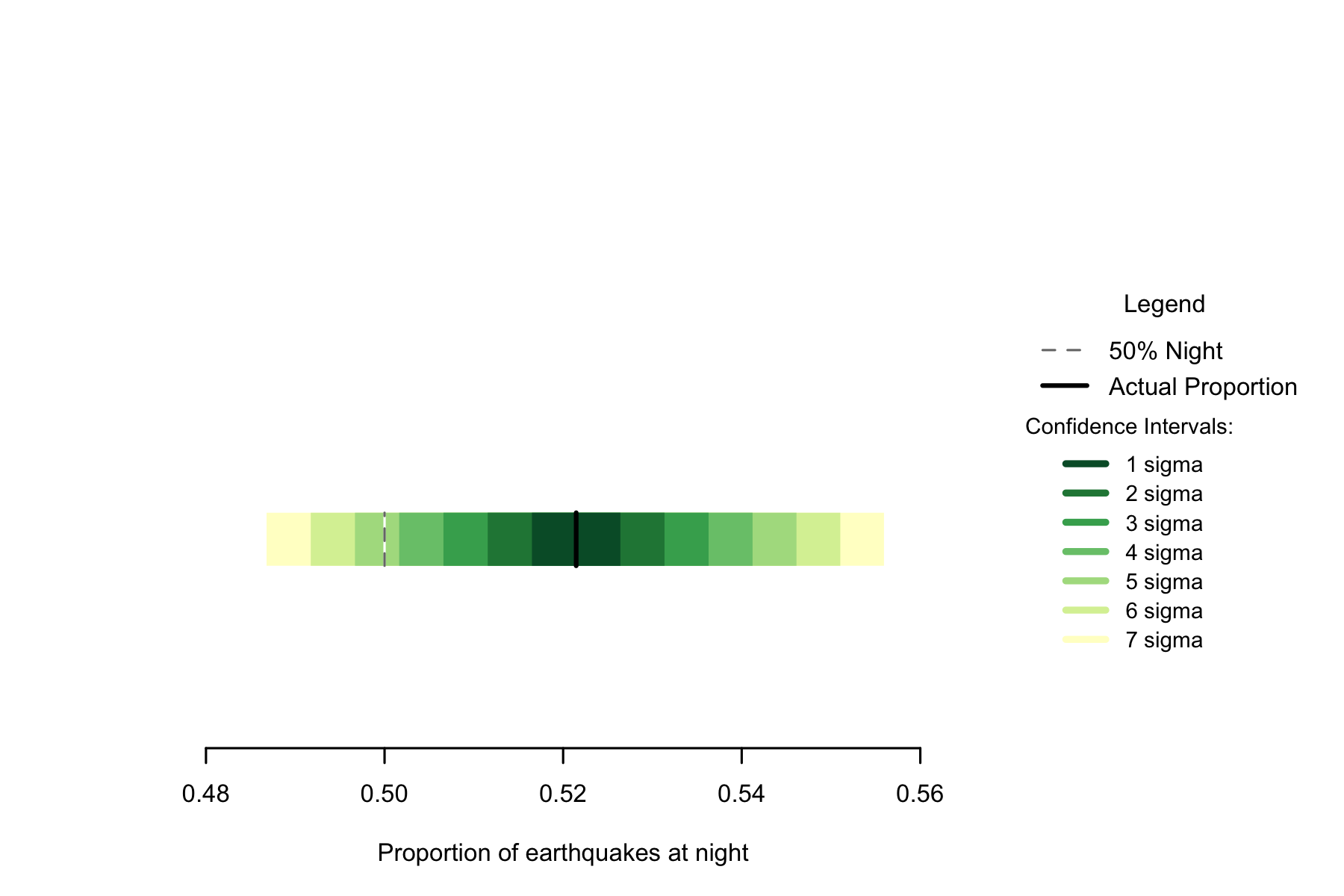
Figure 7.1: Proportion of earthquakes at night: Hawaii. n=10181
While 4 confidence intervals would normally be a significant result in its own right, I can also observe Hawaii has a higher proportion of nighttime earthquakes than the continental United States, it is just that with around 5% the number of earthquakes we are less certain about the exact proportion.
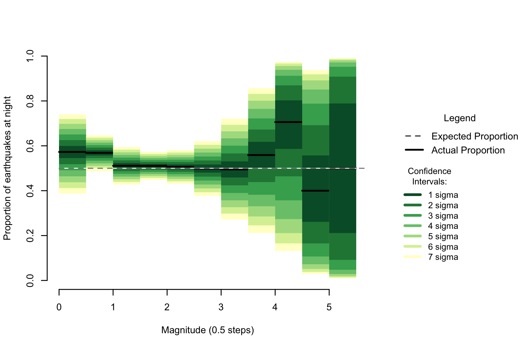
Figure 2.4: Proportion of night earthquakes by magnitude, Hawaii. n=10181
Examining magnitude, there is a similar pattern to New Zealand. Even with the small number of earthquakes, it is clear that earthquakes of a small magnitude are occurring more often at night.
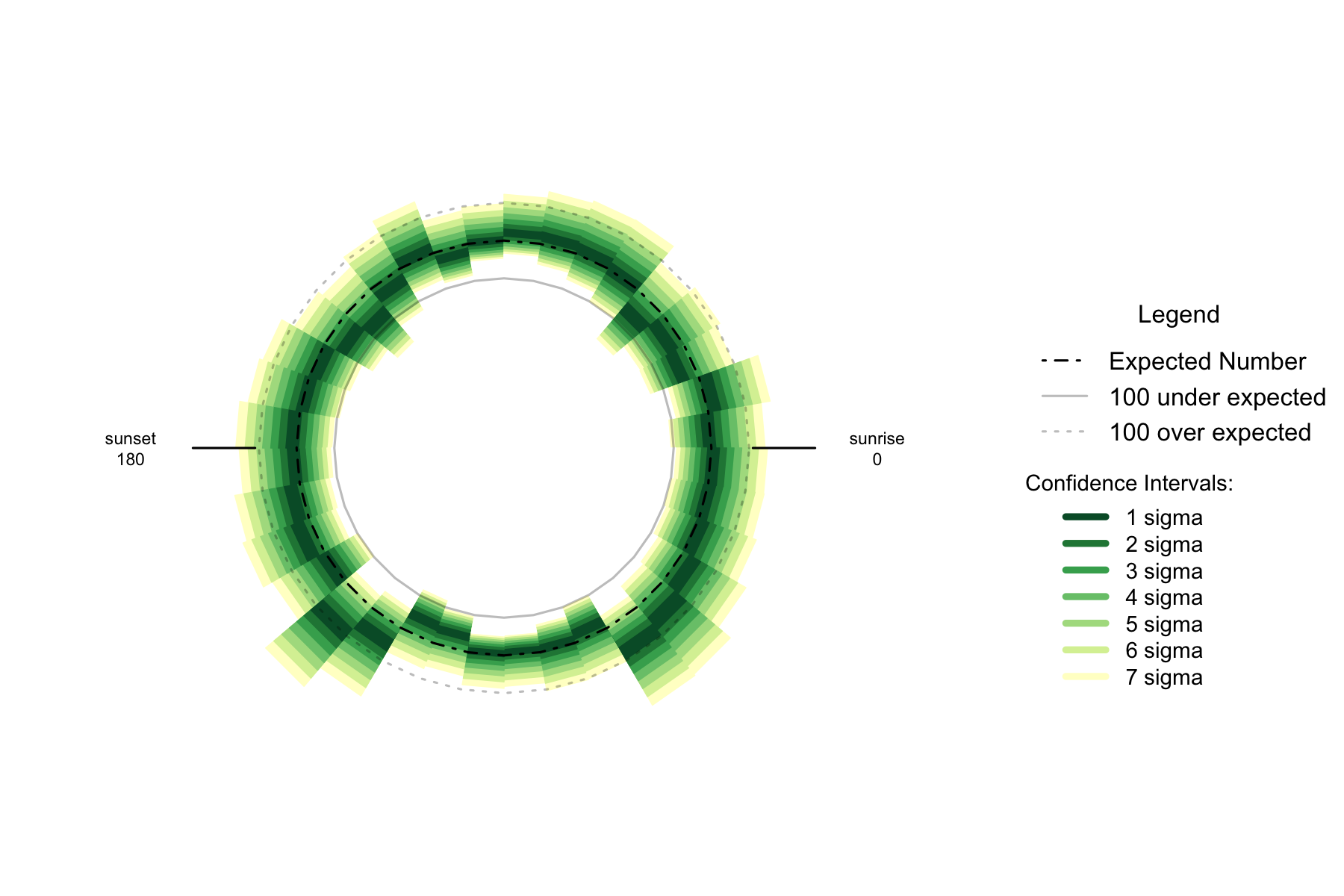
Figure 7.3: Over- and under- supply of earthquakes by angle of the sun (10 degree steps). Hawaii. n=10181
The trend for the number of earthquakes by 10 degree arc of the sun is similar to New Zealand, but much less pronounced. Peak oversupply is around 40 to 50 degrees below the horizon. Peak undersupply is 30 to 50 degrees above the horizon.
12.1 Formal Statement
Earthquakes in the region of Hawaii show a similar pattern to New Zealand, displaying an oversupply of earthquakes at night that is not the result of chance. The magnitude pattern of the oversupply is similar to New Zealand’s pattern, and the pattern with respect to the position of the sun is similar to that of New Zealand. Because of the smaller sample size, Hawaii can be described as not inconsistent with New Zealand, Japan, Continental U.S.A., or Italy
12.2 Links
1 - USGS: https://earthquake.usgs.gov
12.3 Chapter Code
## ----setup, include=FALSE------------------------------------------------
knitr::opts_chunk$set(echo = FALSE)

## ----c10_001, warnings=FALSE, errors=FALSE, message=FALSE----------------
library(geosphere)
library(lubridate, quietly=TRUE)
library(dplyr)
library(binom)
library(ggplot2)
library(maps)
library(mapdata)
library(parallel)
library(readr)
library(plotrix)
library(tidyr)
library(maptools)
Sys.setenv(TZ = "UTC")


## ----warnings=FALSE, errors=FALSE, message=FALSE-------------------------

if(!dir.exists("../othereqdata")){
  dir.create("../othereqdata")
}
if(!file.exists("../othereqdata/eq_hawaii_raw.RData")){
bit1 <- "https://earthquake.usgs.gov/fdsnws/event/1/query.csv?"
bit2 <- "starttime=2011-09-01%2000:00:00&endtime=2016-09-01%2000:00:00&"
bit3 <- "maxlatitude=31.436&minlatitude=13.334&maxlongitude=213.882&"
bit4 <- "minlongitude=177.407&minmagnitude=0&orderby=time"
webaddress <- paste0(bit1, bit2, bit3, bit4)
eqhawaii <- read.csv(webaddress, stringsAsFactors = FALSE)

eqhawaii$time_UTC <- as.POSIXct(gsub("\\..+","",as.character(eqhawaii$time)),
                                format="%Y-%m-%dT%H:%M:%S", tz="UTC")
eq_national <- eqhawaii %>%
  filter(depth > 0 & mag >= 0 &
           time_UTC >= as.POSIXct("2011-09-01T00:00:00",
                                  format="%Y-%m-%dT%H:%M:%S", tz="UTC") &
           time_UTC < as.POSIXct("2016-09-01T00:00:00",
                                 format="%Y-%m-%dT%H:%M:%S", tz="UTC")) %>%
  distinct()  %>% arrange(time_UTC)

rm(eqhawaii)
names(eq_national)[5] <- "magnitude"
save(eq_national, file="../othereqdata/eq_hawaii_raw.RData")
}

## ------------------------------------------------------------------------

if(!file.exists("../othereqdata/eq_hawaii_processed.RData")){
load("../othereqdata/eq_hawaii_raw.RData")
southmost <- min(eq_national$latitude)
westmost <- min(eq_national$longitude)


eq_national <- eq_national %>% filter(
  magnitude > 0, depth > 0) %>% rowwise() %>% mutate(
  eq_gridpoint_y = round(
    distVincentyEllipsoid(c(longitude, southmost),c(longitude,latitude)) /50000,0),
  eq_gridpoint_x = round(
    distVincentyEllipsoid(c(westmost, latitude), c(longitude,latitude)) /50000,0),
  eq_roundedlat = destPoint(
    p=c(longitude, southmost), b=0, d=eq_gridpoint_y*50000)[2],
  eq_roundedlong = destPoint(
    p=c(westmost, eq_roundedlat), b=90, d=eq_gridpoint_x*50000)[1]) %>% ungroup()
# use maptools to calculate solar angles
sun_angles <- solarpos(
  matrix(c(eq_national$longitude, eq_national$latitude), ncol=2), eq_national$time_UTC)
colnames(sun_angles) <- c("eq_compass", "eq_vertical")
eq_national <- cbind(eq_national,sun_angles)
eq_national$eq_is_night <- eq_national$eq_vertical < 0
# calculate 360 degree as well as vertical
eq_national <- eq_national %>%
  mutate(eq_angle_360 = eq_vertical,
         eq_angle_360 = ifelse(eq_compass > 180, 180 - eq_angle_360, eq_angle_360),
         eq_angle_360 = ifelse(eq_vertical < 0 & eq_compass <= 180,
                               360 + eq_angle_360, eq_angle_360),
         eq_angle_by_10 = floor(eq_angle_360 /10) * 10)
save(eq_national, file="../othereqdata/eq_hawaii_processed.RData")
}

## ------------------------------------------------------------------------
if(!file.exists("../othereqdata/eq_hawaii_expected.RData")){
load("../othereqdata/eq_hawaii_processed.RData")

lat_range <- unique(eq_national$eq_roundedlat)
long_med <- median(eq_national$eq_roundedlong)

# 1 minute intervals for a full solar year
time1 <- ymd_hms("2015-01-01 00:00:00")
time2 <- ymd_hms("2015-12-31 23:59:00")
time_sq <- seq.POSIXt(from=time1, to=time2, by="min")


calc_angs <- function(x, longinput, timeinput){
  library(dplyr)
  sun_angles <- maptools::solarpos(matrix(c(longinput, x), ncol=2), timeinput)
  colnames(sun_angles) <- c("eq_compass", "eq_vertical")
# calculate 360 degree as well as vertical
site_summary <- as.data.frame(sun_angles) %>%
  mutate(eq_angle_360 = eq_vertical,
         eq_angle_360 = ifelse(eq_compass > 180, 180 - eq_angle_360, eq_angle_360),
         eq_angle_360 = ifelse(
           eq_vertical < 0 & eq_compass <= 180, 360 + eq_angle_360, eq_angle_360),
         eq_angle_by_10 = floor(eq_angle_360 /10) * 10) %>%
  group_by(eq_angle_by_10) %>% summarise(total= n())
  site_summary$lat <- x
  return(site_summary)
}
###
# Calculate the number of cores
no_cores <- detectCores() - 1
# Initiate cluster
cl <- makeCluster(no_cores)
clusterExport(cl, varlist=c("lat_range", "long_med", "time_sq", "calc_angs"))
list_angs <- parLapply(cl, lat_range,
                         function(x){
                           calc_angs(x=x, longinput=long_med, timeinput=time_sq)})
stopCluster(cl)
###
library(tidyr)
anglong <- bind_rows(list_angs)
angwide <- spread(anglong, key=eq_angle_by_10,value=total)
rm(anglong, list_angs, time_sq)
save(angwide, file="../othereqdata/eq_hawaii_expected.RData")
}

## ------------------------------------------------------------------------
load("../othereqdata/eq_hawaii_processed.RData")
load("../othereqdata/eq_hawaii_expected.RData")
eq_night = sum(eq_national$eq_is_night)
eq_total = nrow(eq_national)
 bands <- rev(c('#ffffcc','#d9f0a3','#addd8e','#78c679','#41ab5d','#238443','#005a32'))
 sigmas <- c(0.682689492137086,
 0.954499736103642,
 0.997300203936740,
 0.999936657516334,
 0.999999426696856,
 0.999999998026825,
 0.999999999997440)
 lbls <- c(
 "1 sigma", "2 sigma",
 "3 sigma", "4 sigma",
 "5 sigma", "6 sigma",
 "7 sigma")
typs <- c(1,1,1,1,1,1,1)
weights <- c(3,3,3,3,3,3,3)
old_par=par()

## ------------------------------------------------------------------------
bt <- binom.test(eq_night ,eq_total, conf.level= .999999999997440)

## ------------------------------------------------------------------------
feature <- c("Earliest (UTC)", "Latest (UTC)",
             "Northernmost", "Southernmost",
             "Westmost", "Eastmost",
             "Percent < Mag 3", "total entries",
             "nighttime quakes")
value <- c(as.character(min(eq_national$time_UTC)),
           as.character(max(eq_national$time_UTC)),
           as.character(max(eq_national$latitude)),
           as.character(min(eq_national$latitude)),
           as.character(max(eq_national$longitude)),
           as.character(max(eq_national$longitude[eq_national$longitude<0])),
           as.character(round(100*sum(eq_national$magnitude < 3)/eq_total,2)),
           as.character(eq_total),
           as.character(eq_night))
data.frame(feature,value) %>% knitr::kable(caption="Data description")

## ---- fig.cap="Proportion of earthquakes at night: Hawaii. n=10181"------
### making the basic proportion graph
eq_night = sum(eq_national$eq_is_night)
eq_total = nrow(eq_national)
bands <- rev(c('#ffffcc','#d9f0a3','#addd8e','#78c679','#41ab5d','#238443','#005a32'))
sigmas <- c(0.682689492137086,
            0.954499736103642,
            0.997300203936740,
            0.999936657516334,
            0.999999426696856,
            0.999999998026825,
            0.999999999997440)
lbls <- c(
  "1 sigma", "2 sigma",
  "3 sigma", "4 sigma",
  "5 sigma", "6 sigma",
  "7 sigma")
typs <- c(1,1,1,1,1,1,1)
weights <- c(3,3,3,3,3,3,3)
old_par=par()
conf_steps <- function(x, sigmas=sigmas, night=eq_night, total=eq_total){
  ci_lower <- binom.confint(night, total, method=c("wilson"), conf.level = sigmas[x])[1,5]
  ci_upper <- binom.confint(night, total, method=c("wilson"), conf.level = sigmas[x])[1,6]
  ci_data <- data.frame(step = x, ci_lower, ci_upper)
}

ci_spacing <- lapply(7:1, conf_steps, sigmas=sigmas, night=eq_night, total=eq_total)
ci_steps <- bind_rows(ci_spacing)

layout(matrix(c(1,1,1,2), ncol=4))

par(mar=c(5,6,4,2))
plot(c(min(0.5,floor(100*ci_steps[1,2])/100), max(0.5,ceiling(100*ci_steps[1,3])/100)),
       y=c(-3,8), type="n", bty="n", yaxt="n", ylab="",
       xlab="Proportion of earthquakes at night")
a <- a <- apply(ci_steps, 1, function(x){
  polygon(c(x[2], x[3], x[3], x[2]), c(0, 0, 1, 1), col=bands[x[1]], border=NA)})
lines(c(.5,.5), c(0,1), col="#FFFFFF")
lines(c(.5,.5), c(0,1), lty=2, col="#777777")
lines(c(eq_night/eq_total,eq_night/eq_total), c(0,1), lwd=2)

par(mar=c(0,0,0,0))
plot(x=c(0,10), y=c(0,10), type="n", bty="n", axes=FALSE)
legend(0,5.5, legend=lbls, lty=typs, lwd=weights, col=bands, bty="n", xjust=0,
       title="Confidence Intervals:", y.intersp=1.1, cex=0.9)

lbls2=c("50% Night", "Actual Proportion")
typs2=c(2,1)
weights2=c(1,2)
cls2=c("#777777","#000000")
legend(0,7, legend=lbls2, lty=typs2, lwd=weights2, col=cls2, bty="n", xjust=0,
       title="Legend", y.intersp=1.2)


par(mar=old_par$mar)
par(mfrow=c(1,1))


## ---- fig.cap="Proportion of night earthquakes by magnitude, Hawaii. n=10181"----
old_par=par()
grf <- eq_national %>% mutate(floored_mag = floor(magnitude*2)/2) %>%
  group_by(floored_mag) %>% summarise(successes = sum(eq_is_night), trials=n())

poly_conf_int <- function(success, trials, aa, stepsize, sigma, colr){
  ci <- binom.confint(success, trials, method=c("wilson"), conf.level = sigma)
  lower <- ci[1,5]
  upper <- ci[1,6]
  a <- polygon(x=c(aa,aa+stepsize,aa+stepsize,aa), y=c(upper,upper,lower,lower),
               col=colr, border=NA)
}


plot7sig <- function(success, trials, aa, stepsize){
  library(binom)
  #bands <- c('#ffffb2','#fed976','#feb24c','#fd8d3c','#fc4e2a','#e31a1c','#b10026')
  bands <- rev(c('#ffffcc','#d9f0a3','#addd8e','#78c679','#41ab5d','#238443','#005a32'))
  sigmas <- c(0.682689492137086,
              0.954499736103642,
              0.997300203936740,
              0.999936657516334,
              0.999999426696856,
              0.999999998026825,
              0.999999999997440)
  sapply(7:1, function(x){
    poly_conf_int(success, trials, aa, stepsize, sigmas[x], bands[x])})
  a <- lines(c(aa, aa + stepsize), c(success/trials, success/trials), lwd=2)
}


lbls <- c(
  "1 sigma", "2 sigma",
  "3 sigma", "4 sigma",
  "5 sigma", "6 sigma",
  "7 sigma")
typs <- c(1,1,1,1,1,1,1)
weights <- c(3,3,3,3,3,3,3)
clrs <- rev(c('#ffffcc','#d9f0a3','#addd8e','#78c679','#41ab5d','#238443','#005a32'))
#clrs <- c('#ffffb2','#fed976','#feb24c','#fd8d3c','#fc4e2a','#e31a1c','#b10026')

layout(matrix(c(1,1,1,2), ncol=4))
plot(x=c(0,max(grf$floored_mag)+0.5), y=c(0,1), type="n", bty="n",
     xlab="Magnitude (0.5 steps)", ylab="Proportion of earthquakes at night")
a <- apply(grf,1,function(x){plot7sig(x[2],x[3],x[1],0.5)})
lines(c(0,10), c(.5,.5), col="#FFFFFF")
lines(c(0,10), c(.5,.5), lty=2, col="#777777")

par(mar=c(0,0,0,0))
plot(x=c(0,10), y=c(0,10), type="n", bty="n", axes=FALSE)
legend(0,5, legend=lbls, lty=typs, lwd=weights, col=clrs, bty="n", xjust=0,
       title="Confidence
Intervals:", cex=0.9)
lbls=c("Expected Proportion", "Actual Proportion")
typs=c(2,1)
weights=c(1,2)
legend(0,7, legend=lbls, lty=typs, lwd=weights, bty="n", xjust=0,
       title="Legend", y.intersp=1.2)


par(mar=old_par$mar)
par(mfrow=c(1,1))


## ------------------------------------------------------------------------
by_angle <- eq_national %>%
  group_by(eq_angle_by_10) %>% summarise(total= n()) %>%
  mutate(daynight=ifelse(eq_angle_by_10 < 180, "day", "night"))

merged <- merge(eq_national, angwide, by.x="eq_roundedlat", by.y="lat")
agg_expected <- merged %>% select(`0`:`350`) %>% colSums(na.rm=TRUE)
expected_prop <- agg_expected / sum(agg_expected)
expected <- data.frame(eq_angle_by_10 = as.numeric(names(expected_prop)),
                       expected_prop = as.numeric(expected_prop))
expected$expected_number = expected_prop * eq_total
act_exp <- merge(expected, by_angle, by="eq_angle_by_10", all.x=TRUE)

act_exp$total[is.na(act_exp$total)] <- 0
act_exp$daynight <- NULL
act_exp$act_prop <- act_exp$total / sum(act_exp$total)


ci_brackets <- act_exp %>% ungroup() %>% mutate(grand_total=sum(total)) %>%
  rowwise() %>% mutate(
    ci_lower_7 = binom.confint(total, grand_total, method=c("wilson"),
                               conf.level = sigmas[7])[1,5] * grand_total,
    ci_upper_7 = binom.confint(total, grand_total, method=c("wilson"),
                               conf.level = sigmas[7])[1,6] * grand_total,
    ci_lower_6 = binom.confint(total, grand_total, method=c("wilson"),
                               conf.level = sigmas[6])[1,5] * grand_total,
    ci_upper_6 = binom.confint(total, grand_total, method=c("wilson"),
                               conf.level = sigmas[6])[1,6] * grand_total,
    ci_lower_5 = binom.confint(total, grand_total, method=c("wilson"),
                               conf.level = sigmas[5])[1,5] * grand_total,
    ci_upper_5 = binom.confint(total, grand_total, method=c("wilson"),
                               conf.level = sigmas[5])[1,6] * grand_total,
    ci_lower_4 = binom.confint(total, grand_total, method=c("wilson"),
                               conf.level = sigmas[4])[1,5] * grand_total,
    ci_upper_4 = binom.confint(total, grand_total, method=c("wilson"),
                               conf.level = sigmas[4])[1,6] * grand_total,
    ci_lower_3 = binom.confint(total, grand_total, method=c("wilson"),
                               conf.level = sigmas[3])[1,5] * grand_total,
    ci_upper_3 = binom.confint(total, grand_total, method=c("wilson"),
                               conf.level = sigmas[3])[1,6] * grand_total,
    ci_lower_2 = binom.confint(total, grand_total, method=c("wilson"),
                               conf.level = sigmas[2])[1,5] * grand_total,
    ci_upper_2 = binom.confint(total, grand_total, method=c("wilson"),
                               conf.level = sigmas[2])[1,6] * grand_total,
    ci_lower_1 = binom.confint(total, grand_total, method=c("wilson"),
                               conf.level = sigmas[1])[1,5] * grand_total,
    ci_upper_1 = binom.confint(total, grand_total, method=c("wilson"),
                               conf.level = sigmas[1])[1,6] * grand_total)

norm_ci <- ci_brackets

for (i in c(4,7:20)){
norm_ci[,i] <- ci_brackets[,i] - ci_brackets[,3]
}
circlesize=100

## ---- fig.cap="Over- and under- supply of earthquakes by angle of the sun
## (10 degree steps). Hawaii. n=10181"----
norm_ci$border = 2
# need to double entries with a displacement of 10
# to make each side of the item on the graph
norm_ci2 <- norm_ci
norm_ci2$eq_angle_by_10 <- norm_ci2$eq_angle_by_10  + 10
norm_ci2$border = 1
graphdata <-   bind_rows(norm_ci,norm_ci2) %>% arrange(eq_angle_by_10,border)

#### plot graph
bands <- rev(c('#ffffcc','#d9f0a3','#addd8e','#78c679','#41ab5d','#238443','#005a32'))
old_par=par()
layout(matrix(c(1,1,1,2), ncol=4))

# overall limits
limits=2 * max(abs(c(graphdata$ci_lower_7, graphdata$ci_upper_7)))
# plot upper confidence 7 interval using plotrix
polar.plot(graphdata$ci_upper_7, polar.pos=graphdata$eq_angle_by_10,
           radial.lim=c(-1*limits,limits),
           labels = "", main=NULL,lwd=0.5, rp.type="p",
           show.grid.labels=FALSE, show.grid=FALSE, mar=c(0,0,0,0),
           grid.col=bands[7], line.col=bands[7], poly.col=bands[7])
# plot upper 6 confidence interval
plot_ci_round <- function(upper_bound,x){
  polar.plot(upper_bound, polar.pos=graphdata$eq_angle_by_10, add=TRUE,
             radial.lim=c(-1*limits,limits),
             line.col=bands[x], lwd=0.5, rp.type="p", poly.col=bands[x])
}
plot_ci_round(graphdata$ci_upper_6, 6)
plot_ci_round(graphdata$ci_upper_5, 5)
plot_ci_round(graphdata$ci_upper_4, 4)
plot_ci_round(graphdata$ci_upper_3, 3)
plot_ci_round(graphdata$ci_upper_2, 2)
plot_ci_round(graphdata$ci_upper_1, 1)
plot_ci_round(graphdata$ci_lower_1, 2)
plot_ci_round(graphdata$ci_lower_2, 3)
plot_ci_round(graphdata$ci_lower_3, 4)
plot_ci_round(graphdata$ci_lower_4, 5)
plot_ci_round(graphdata$ci_lower_5, 6)
plot_ci_round(graphdata$ci_lower_6, 7)
polar.plot(graphdata$ci_lower_7, polar.pos=graphdata$eq_angle_by_10,
           add=TRUE, radial.lim=c(-1*limits,limits),
           line.col="white", lwd=0.5, rp.type="p", poly.col="white")

# plot expected guide line
polar.plot(rep(0,nrow(graphdata)), polar.pos=graphdata$eq_angle_by_10, add=TRUE,
           radial.lim=c(-1*limits,limits),
           rp.type="p", lty=4)
# plot 500 less than expected guide line
polar.plot(rep(-1 * circlesize,nrow(graphdata)), polar.pos=graphdata$eq_angle_by_10,
           add=TRUE,radial.lim=c(-1*limits,limits),
           rp.type="p", lty=1, line.col="#00000044")
# plot 500 more than expected guide line
polar.plot(rep(circlesize,nrow(graphdata)), polar.pos=graphdata$eq_angle_by_10,
           add=TRUE,radial.lim=c(-1*limits,limits),
           rp.type="p", lty=3, line.col="#00000044")

lines(c(-1.5,-1.2)*limits, c(0,0))
lines(c(1.5,1.2)*limits, c(0,0))
text(-1.8*limits,0, label="sunset
180", cex=0.7)
text(1.8*limits,0, label="sunrise
0", cex=0.7)


par(mar=c(0,0,0,0))
plot(x=c(0,10), y=c(0,10), type="n", bty="n", axes=FALSE, xlab="")
lbls <- c(
  "1 sigma", "2 sigma",
  "3 sigma", "4 sigma",
  "5 sigma", "6 sigma",
  "7 sigma")
typs <- c(1,1,1,1,1,1,1)
weights <- c(3,3,3,3,3,3,3)
clrs <- rev(c('#ffffcc','#d9f0a3','#addd8e','#78c679','#41ab5d','#238443','#005a32'))
legend(0,4.5, legend=lbls, lty=typs, lwd=weights, col=clrs, bty="n", xjust=0,
       title="Confidence Intervals:", cex=0.9)

lbls2=c("Expected Number", paste(circlesize,"under expected"),
        paste(circlesize,"over expected"))
typs2=c(4,1,3)
weights2=c(1,1,1)
clrs2=c("#000000","#00000044","#00000044")
legend(0,10, legend=lbls2, lty=typs2, lwd=weights2, bty="n", xjust=0,
       title="Legend", y.intersp=1.2, col=clrs2)


par(mar=old_par$mar)
par(mfrow=c(1,1))