Chapter 2 Data Processing

Data processing involves finding, and ideally fixing, problems in the data that prevent an analysis being made. It also involves inventing transformations in the data to allow new insights. To me, the first of these is largely a matter of practice in becoming familiar with what goes wrong with data. The second is a more creative process of “what can be done to the data to get it to reveal things it otherwise would not, and is there a price to be paid in doing so?”

A good place to start is to make some general summaries looking for any odd biases in the data.

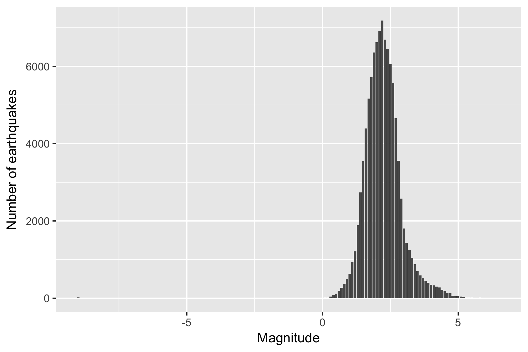
Figure 2.1: Distribution of Magnitude (steps of .1)

This is an artificially normal looking distribution. To the right of the peak of the histogram, at about magnitude 2.2, the number of earthquakes are decreasing as earthquakes become less frequent at higher magnitudes. To the left of the peak, the number is decreasing due to smaller earthquakes being more difficult to detect. This missing data might cause potential biases in the results if there is a connection between an earthquake being detected at all and the time that it was detected.

In checking, there are a small number of events of -9 magnitude (negative magnitude is possible but rare). These seem to be extreme outliers and are likely to badly affect any model I create (as well as cause annoying amounts of empty space on graphs of magnitude).

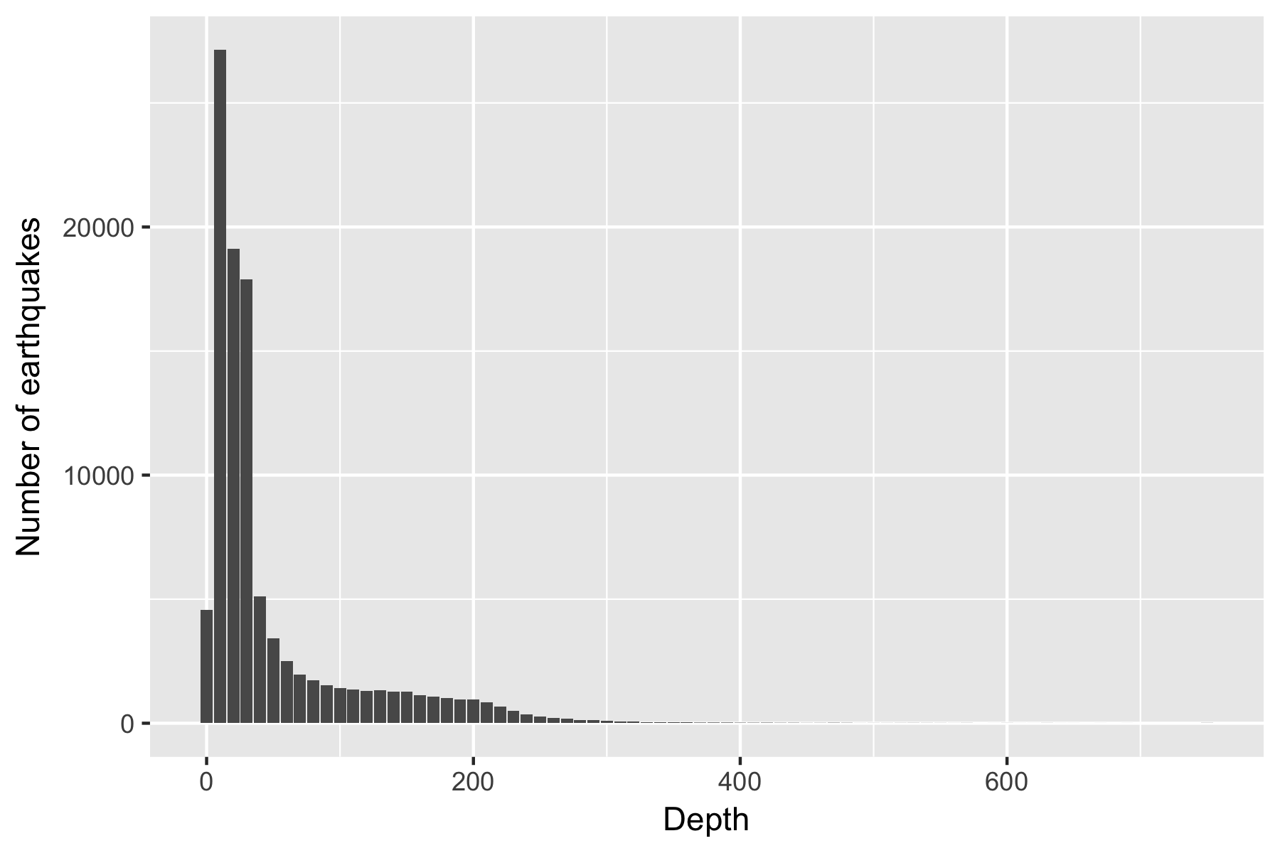
Figure 1.1: Distribution of Depth (steps of 10 km)

The graph of estimated earthquake depth does not have a smooth distribution; it is worth nothing that the earth’s crust is not smoothly distributed either, so this is unsurprising. There is an unusual reduction in events around depth 0. This is as much an excuse not to include events at this depth as a reason; the mechanics of bits of ground pushing and pulling against other bits of ground feels like it should be different at surface level, and on that basis alone I am happy to put surface events to one side

From the exploratory analysis this far I am inclined to:

remove events of less than zero magnitude as being very few and suspiciously different to the rest of the data
remove surface events as being different to subsurface ones.

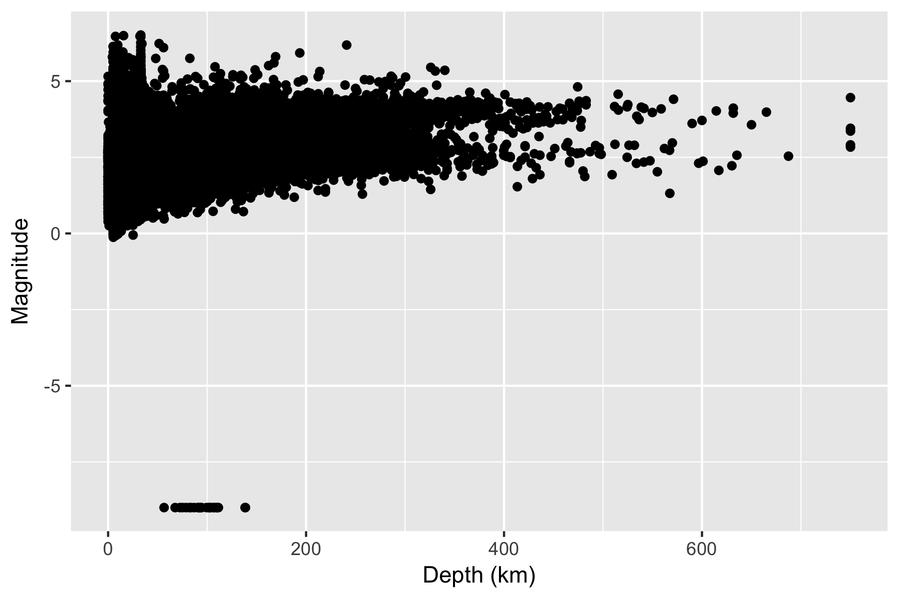
Figure 2.2: Depth and Magnitude of earthquakes

From the graph of magnitude vs depth I see no reason to keep either the surface earthquakes or the negative magnitude earthquakes. In this I am technically not following best practice; since neither group of earthquakes affect the overall analysis, it would be better practice to keep them in (those comfortable in modifying the code I provide can easily discover the inclusion of these earthquakes makes no difference to the conclusions). Best practice would be to include the most data to make the broadest conclusions. However, I personally do not want to get bogged down in comparatively trivial debates about the quality of the data with the negative magnitude earthquakes included, or the interplay of forces with surface level earthquakes, so I am personally happy to discuss things in terms of positive magnitude subsurface earthquakes.

After removing the events at the surface and the events below zero magnitude, I did a quick check of what the magnitude distributions for under 3 magnitude earthquakes look like for each hour of the day. Magnitudes of under three were chosen because that is the level at which the number of detectable earthquakes begins to decrease, and therefore the missing data could cause biases.

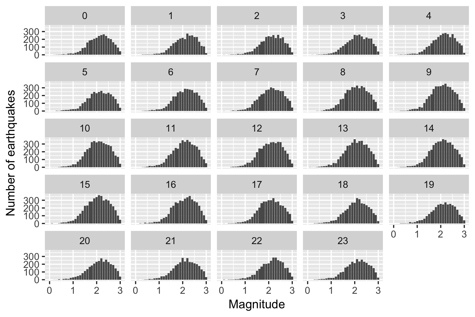
Figure 2.3: Number of earthquakes by magnitude, split by hour of day (UTC)

All the individual hours seem to be showing a similar pattern, which leads me (in judging it by eye) to suspect it will be unlikely that there is any relationship between detected earthquakes and time of day that could be influencing results.

2.1 Event types

From the Earthquake Catalogue documentation, I am interested in two classes of events: earthquakes (reviewed by a human being) and likely earthquakes (indicated by a blank entry, but as that is annoying in tables I am replacing it with the term “likely earthquake” in the data)

Table 2.1: Events types and number in the Geonet Database
Event type	Total
duplicate	1
earthquake	36424
explosion	1
induced earthquake	1
landslide	1
likely earthquake	63855
not locatable	19
nuclear explosion	1
other	1
outside of network interest	1367
quarry blast	21
volcanic eruption	1

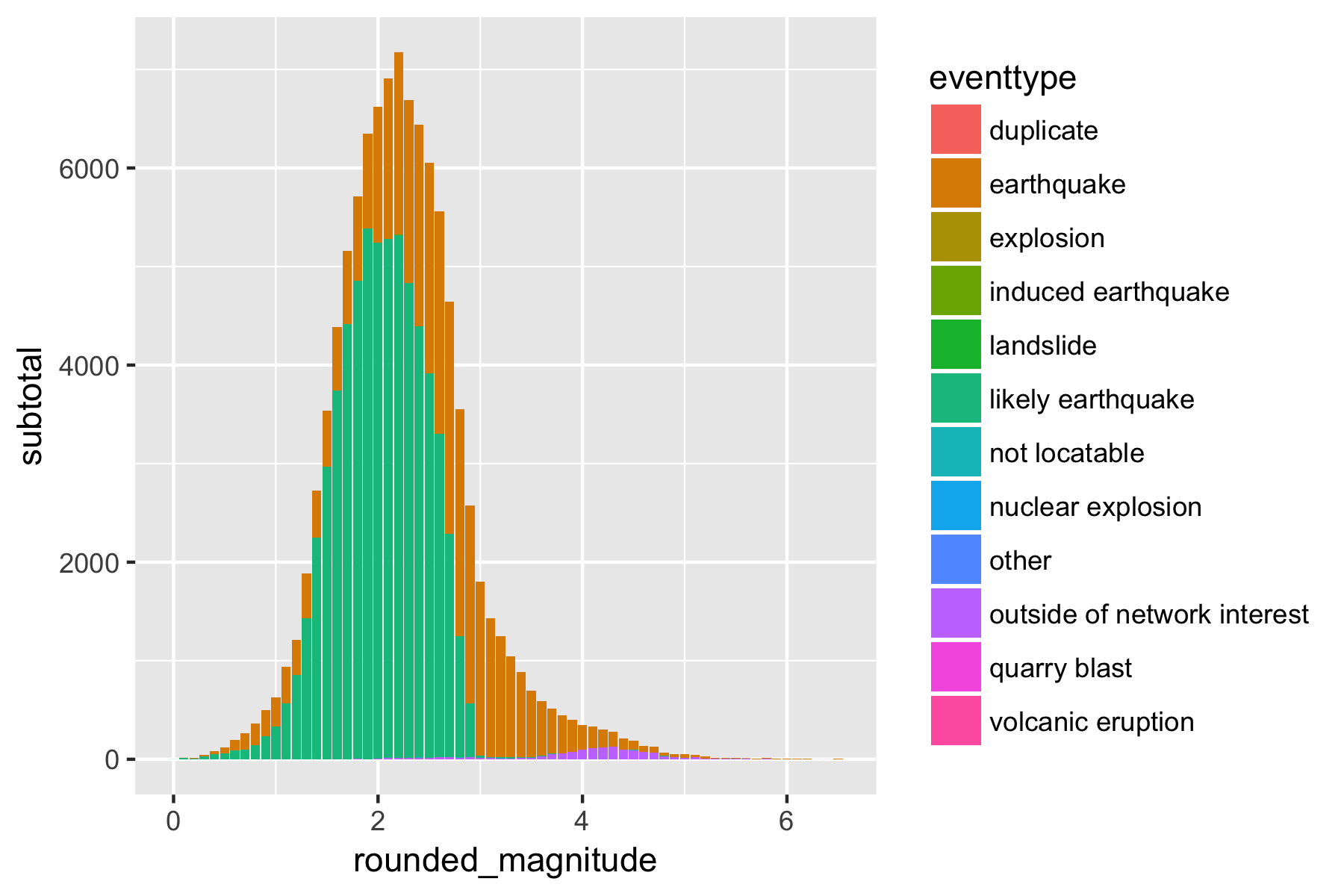
Figure 2.4: Number of earthquakes by Magnitude and Classification

This human review process could, in theory, mean that there are unknown confounders causing a large number of low magnitude events. However, there are no significant numbers of non-earthquake classified events with a magnitude of less than three, so there is no evidence for any alternative. As a result, I am agreement with the Geonet documentation that likely earthquakes can be considered earthquakes.

2.1.1 Latitude and Longitude

Latitude and longitude are critical to the analysis, so it seems like a good idea to actually check them, particularly since New Zealand is near the international date line with a sudden longitude shift from 180 to -180.

Latitudes range from -49.3178902 to -32.4753952, while longitudes range from -179.9998322 to 180.63854 (thought it might be better to say longitudes from 164.2942963 to -177.59093).

The presence of negative longitudes represented as positive numbers greater than 180 causes problems for some R packages when conducting longitude related calculations, so I will correct the greater than 180 values to be negative values slightly greater than -180.

From the raw earthquake data I calculate a series of out variables, mostly following the principle of “it seemed like a good idea at the time”.

2.2 Gridded Latitude and Longitude

In the raw data, the earthquakes are individual events, but another way of looking at the data is as regions which have earthquakes. One straightforward approach is to take the entire area represented by the data, and divided that area into grids.

The size of the grids is a trade-off. Larger grids mean that local differences are homogenised into one block and variation between smaller in-block areas is lost. In this view, the analysis of the entire data is an analysis of one large grid square. On the other hand, smaller areas reduce the number of earthquakes in any single area, reducing the sample size and therefore weakening our confidence in our statistical results. An individual earthquake by itself is representative of a tiny area. An initial grid composed of squared 50km on a side seems reasonable here, given the size of the total area and the number of earthquakes within the 5 year period.

To make the grids, I found the southernmost of the earthquake events and calculate how far north of that base point each earthquake is. Then divided that distance by 50 and rounded to a whole number. I converted that distance back to a latitude for convenience of future plotting.

I take the same approach for longitude, starting from the easternmost earthquake and working westwards to calculate the grid centre closest to the earthquake event location.

While I might feel that 50 kilometres per side is a good grid size, I should also verify this intuition using tests:

104 (28%) of the 377 grid locations have more than 100 earthquakes, which I would expect to be enough to draw useful conclusions from, as each grid point contributes less than 1% to the overall figures. Each earthquake in each grid square also contributes less than 1% to the overall aggregate for the square. Among the data that we have, this minimises the effects of unusual variation.

2.3 Angle of the sun

Using the hour of the day is only an approximate measure of night and day, as the position of the sun at a particular hour changes with latitude, longitude, and time of year. Exactly declaring a particular place and time night or day requires knowing the position of the sun at that moment. This can be done with a function in the maptools package. The function returns both a compass and vertical angle for the sun’s position, and I convert that to a 360 degree angle along an east-west arc. My reason for doing so is that the east-west arc of the sun sees the significant daily change, while the north-south component is a gradual seasonal change. This, in turn, allows me to simplify the problem from a three-dimensional one to a two-dimensional problem focused on the change within a day.

At the same time, I can use time of sunrise and sunset to calculate the length of night in the day the earthquake took place on, as this can be a better measure for seasonality than month, since the months cycle is slightly offset from the solar cycle of around 21st of December to 21st of June.

From the help files for the solar position function, the N.O.A.A. provided algorithms are accurate to approximately one minute for sunrise and sunset among latitudes with +/- 72 degrees.

Given there is a tiny potential uncertainty, I carry out quick test that it is giving sensible answers, by checking the range of sun angles per hour of UTC day.

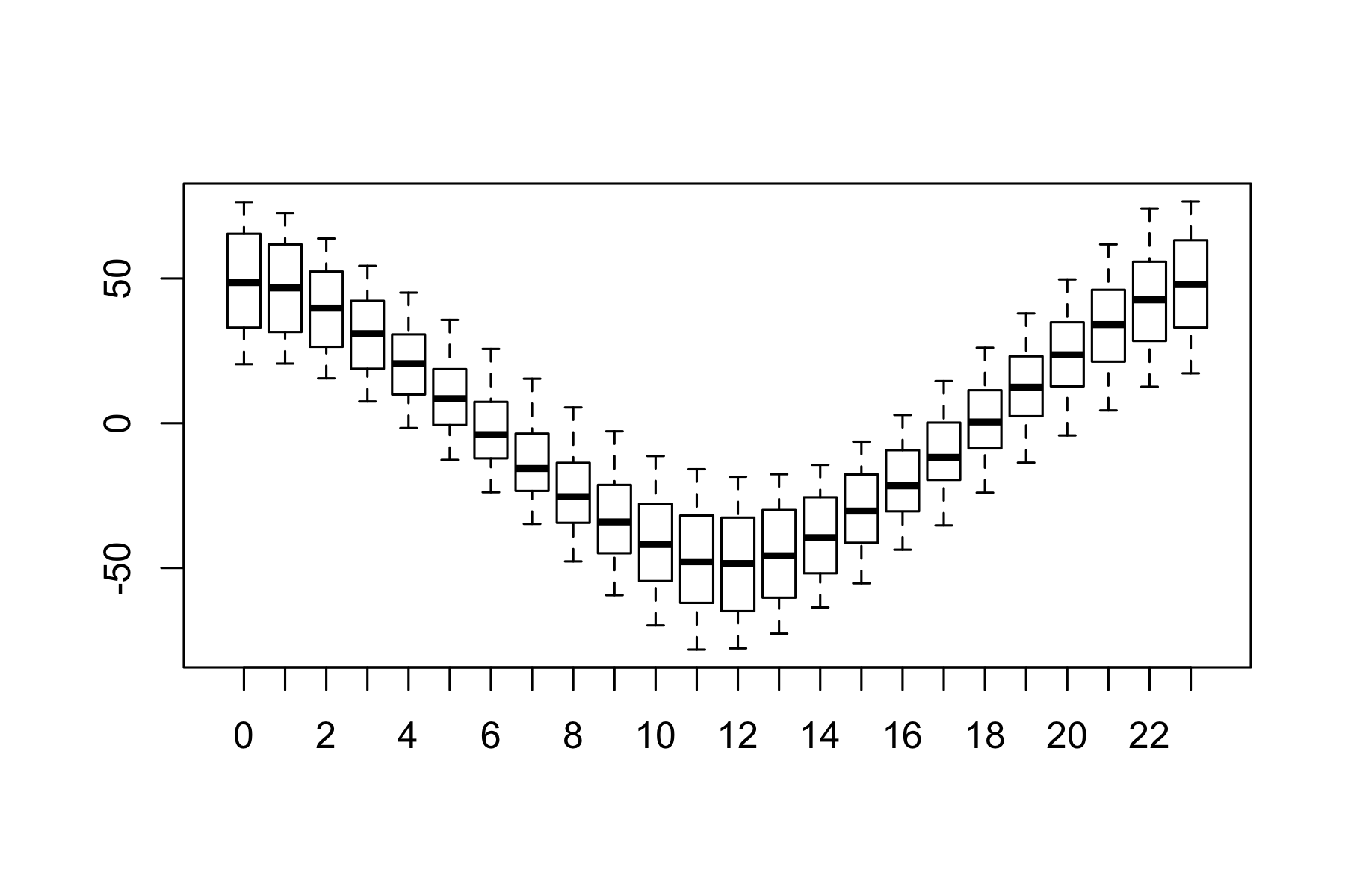
Figure 2.5: Variation in angle of sun by hour of day

The range of values seems reasonable, so I have no concerns about the calculated angles.

2.4 Formal statement

This analysis is restricted to subsurface earthquake and likely earthquake events of greater than zero magnitude.

2.5 Code

2.6 Chapter Code

## ----setup, include=FALSE------------------------------------------------
knitr::opts_chunk$set(echo = FALSE)
knitr::opts_chunk$set(warnings=FALSE)
knitr::opts_chunk$set(errors=FALSE)
knitr::opts_chunk$set(message=FALSE)
knitr::opts_chunk$set(dpi = 150)
knitr::opts_chunk$set(fig.width =  6)
knitr::opts_chunk$set(fig.height =  4)

## ------------------------------------------------------------------------
library(dplyr)
library(lubridate)
library(ggplot2)
library(maptools)
library(geosphere)
library(solidearthtide)
Sys.setenv(TZ = "UTC") 

# Assumes there is eqnz_raw data created in chapter 1
load("eqdata/eqnz_raw.RData")

## ----fig.cap="Distribution of Magnitude (steps of .1)"-------------------
eqnz %>% mutate(rounded_magnitude=round(magnitude,1)) %>% 
  group_by(rounded_magnitude) %>%
  summarise(subtotal = n()) %>% 
  ggplot(aes(x=rounded_magnitude, y=subtotal)) + geom_bar(stat="identity") +
  ylab("Number of earthquakes") + xlab("Magnitude")

## ----fig.cap="Distribution of Depth (steps of 10 km)"--------------------
eqnz %>% mutate(rounded_depth=round(depth,-1)) %>% 
  group_by(rounded_depth) %>%
  summarise(subtotal = n()) %>% 
  ggplot(aes(x=rounded_depth, y=subtotal)) + geom_bar(stat="identity") +
  ylab("Number of earthquakes") + xlab("Depth")

## ----fig.cap="Depth and Magnitude of earthquakes"------------------------
ggplot(eqnz, aes(x=depth, y=magnitude)) + geom_point() +
  ylab("Magnitude") + xlab("Depth (km)")

## ----fig.cap="Number of earthquakes by magnitude, split by hour of day (UTC)"----
eqnz %>% filter(magnitude > 0, magnitude < 3) %>%
  mutate(rounded_magnitude=round(magnitude,1), eq_hour = hour(time_UTC)) %>% 
  group_by(rounded_magnitude, eq_hour) %>%
  summarise(subtotal = n()) %>% 
  ggplot(aes(x=rounded_magnitude, y=subtotal)) + geom_bar(stat="identity") + 
  facet_wrap(~ as.factor(eq_hour)) + ylab("Number of earthquakes") +
  xlab("Magnitude")


## ------------------------------------------------------------------------
eqnz$eventtype[eqnz$eventtype == ""] <- "likely earthquake"

## ------------------------------------------------------------------------
eqnz %>% filter(magnitude > 0, depth > 0) %>%
  group_by(eventtype) %>% summarise(total=n()) %>% 
  select(`Event type`=eventtype, Total=total) %>%
  knitr::kable(caption = "Events types and number in the Geonet Database") 

## ----fig.cap="Number of earthquakes by Magnitude and Classification"-----
eqnz %>% filter(magnitude > 0, depth > 0) %>%
  mutate(rounded_magnitude=round(magnitude,1)) %>% 
  group_by(rounded_magnitude, eventtype) %>%
  summarise(subtotal = n()) %>% 
  ggplot(aes(x=rounded_magnitude, y=subtotal, fill=eventtype)) +
  geom_bar(stat="identity")

## ------------------------------------------------------------------------

# only do all the work if work is not done
# to make calculated variables clear, I name them with an eq_prefix

if (!file.exists("eqdata/eqnz_processed.RData")){
eqnz$eventtype[eqnz$eventtype == ""] <- "likely earthquake"
eqnz$longitude[eqnz$longitude > 180] <- eqnz$longitude[eqnz$longitude > 180] - 360
southmost <- min(eqnz$latitude)
westmost <- min(eqnz$longitude[eqnz$longitude > 0])

eqnz <- eqnz %>% filter(
  magnitude > 0, depth > 0, eventtype %in% c("earthquake", "likely earthquake")
) %>% rowwise() %>% mutate(
  eq_gridpoint_y = round(distVincentyEllipsoid(c(longitude, southmost),
                                               c(longitude,latitude)) /50000,0),
  eq_gridpoint_x = round(distVincentyEllipsoid(c(westmost, latitude),
                                               c(longitude,latitude)) /50000,0),
  eq_roundedlat = destPoint(p=c(longitude, southmost),
                            b=0, d=eq_gridpoint_y*50000)[2],
  eq_roundedlong = destPoint(p=c(westmost, eq_roundedlat),
                             b=90, d=eq_gridpoint_x*50000)[1]) %>% ungroup()
# use maptools to calculate solar angles
sun_angles <- solarpos(matrix(c(eqnz$longitude, eqnz$latitude), ncol=2), eqnz$time_UTC)
colnames(sun_angles) <- c("eq_compass", "eq_vertical")
eqnz <- cbind(eqnz,sun_angles)
eqnz$eq_is_night <- eqnz$eq_vertical < 0
# calculate 360 degree as well as vertical
eqnz <- eqnz %>% mutate(
  eq_angle_360 = eq_vertical,
  eq_angle_360 = ifelse(eq_compass > 180, 180 - eq_angle_360, eq_angle_360),
  eq_angle_360 = ifelse(eq_vertical < 0 & eq_compass <= 180, 
                        360 + eq_angle_360, eq_angle_360),
  eq_angle_by_10 = floor(eq_angle_360 /10) * 10)
# get length of night earthquake in hours for UTC day occured in
sunr <- sunriset(matrix(c(eqnz$longitude, eqnz$latitude), ncol=2),
                 eqnz$time_UTC, direction="sunrise", POSIXct.out=TRUE)
suns <- sunriset(matrix(c(eqnz$longitude, eqnz$latitude), ncol=2),
                 eqnz$time_UTC, direction="sunset", POSIXct.out=TRUE)
eqnz$eq_nightlength = 24 - as.numeric(suns$time - sunr$time)
#calculating the solid earth tide vertical component 
soletide_date <- Datenum(as.Date(eqnz$time_UTC)) + 
  (hour(eqnz$time_UTC) * 3600 + minute(eqnz$time_UTC)*60 * second(eqnz$time_UTC))/86400
etv <- Earthtide(eqnz$latitude, eqnz$longitude, soletide_date)
eqnz$eq_solidearth_vertical <- (t(etv))[,1]
save(eqnz, file="eqdata/eqnz_processed.RData")

rm(list=ls())
}
load("eqdata/eqnz_processed.RData")

## ------------------------------------------------------------------------
grid_summary <- eqnz %>% group_by(eq_roundedlat, eq_roundedlong) %>% 
  summarise(subtotal=n()) %>% ungroup() %>% 
  summarise(above_100 = sum(subtotal > 100), total=n())
n_above100 <- grid_summary$above_100[1]
total_grids <- grid_summary$total[1]

## ----fig.cap="Variation in angle of sun by hour of day"------------------
boxplot(eqnz$eq_vertical ~ hour(eqnz$time_UTC))