Chapter 9 Japanese earthquakes are the same
One concern expressed to me is that even if it is a genuine effect, it might just be a New Zealand quirk, rather than a global effect.
A replication in science is when you conduct the same analysis with different data, and see if you reach a similar conclusion. Providing I have earthquake time, location, and magnitude it is easy to repeat the analysis as I just rerun the computer code, and there are many countries that have independently gathered their own earthquake data on their own seismographs. The main way I chose countries was that I could easily find the earthquake collections with an English language web search.
Japan is the source of the best, most detailed, earthquake data. To access the earthquake catalogue, you must register(Link 1), and can then download earthquake information. If you do download 5 years of earthquake data by requesting seven days of earthquakes and saving the web page result, the code is an example of extracting and combining the earthquake data to form a five year set for all Japan.
For the same period as the New Zealand Data (from September 2011 to September 2016) Earthquakes data from the Japan Meteorological Agency, there are 719348 events of depth greater than 0 and magnitude greater than 0.
| feature | value |
|---|---|
| Earliest (UTC) | 2011-09-01 00:02:10 |
| Latest (UTC) | 2016-08-31 23:58:56 |
| Northernmost | 54.007 |
| Southernmost | 18.335 |
| Westmost | 120.1 |
| Eastmost | 158.506 |
| Percent < Mag 3 | 94.47 |
| total entries | 719348 |
| nighttime quakes | 385156 |
Of the 719348 in the data, 385156 occurred at night, a proportion of 0.5354. A seven sigma confidence interval for the proportion of earthquakes occurring at night would be 0.5313 to 0.5395. This confidence interval in no way coincides with 0.5, and using one so large we can confidently say that if earthquakes occur randomly, this result would never occur.
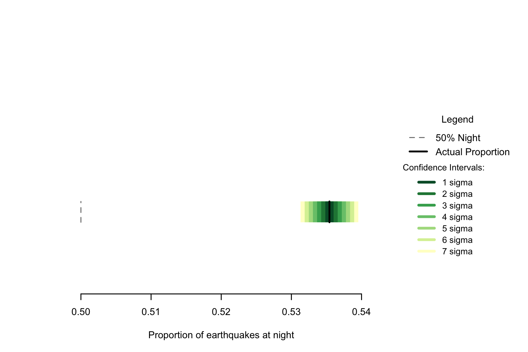
Figure 2.4: Proportion of earthquakes at night: Japan. n=719348
While the proportion is not as high as New Zealand’s, the greater number of earthquakes means that the confidence intervals are smaller, so there is more certainty that the rate of night earthquakes is not 50%
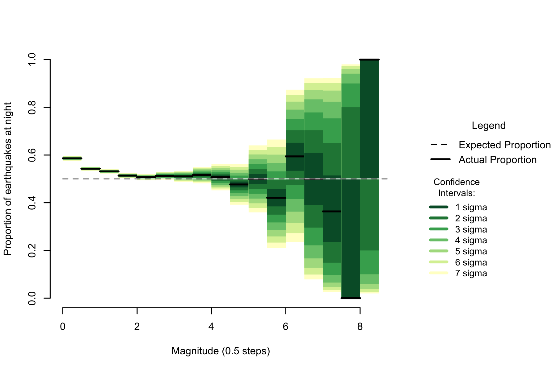
Figure 7.2: Proportion of night earthquakes by magnitude, Japan. n=719348
Examining magnitude, there is a similar pattern to New Zealand. Unequivocally high numbers of earthquakes in the low magnitudes falling towards 50% as magnitude increases, then becoming unclear as sample size decreases.
Taking the expected, and calculating the angle by 10s, and the day night slope.
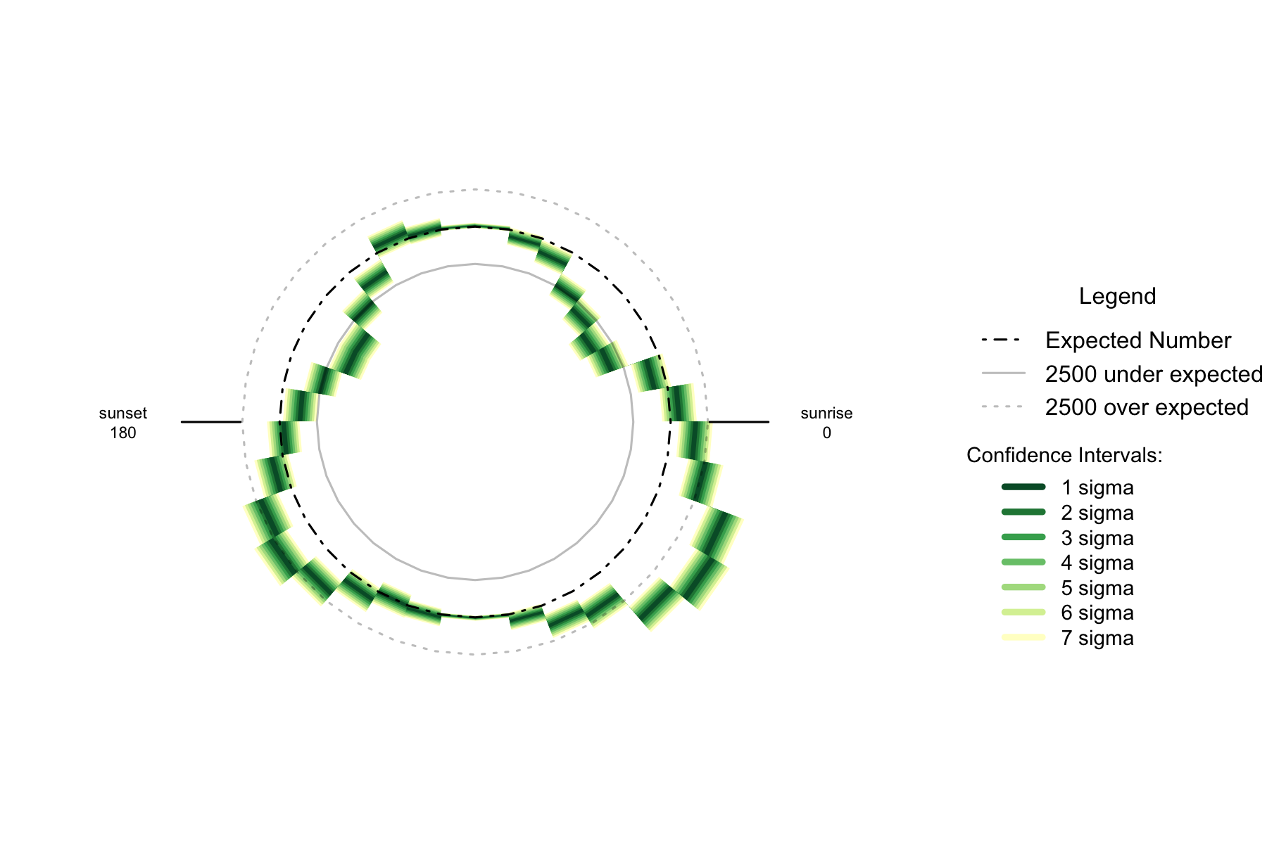
Figure 2.5: Over- and under- supply of earthquakes by angle of the sun (10 degree steps). Japan. n=719348
The trend for the number of earthquakes by 10 degree arc of the sun is similar to New Zealand- undersupplies at 30 degrees above the horizon and oversupplies 30-40 degrees below the horizon. The Japanese data is skewed slightly compared to New Zealand, as the oversupply is clearly at its greatest when the sun is 30 to 40 degrees below the horizon to the east.
9.1 Formal Statement
Earthquakes in Japan show the same pattern as New Zealand, displaying an oversupply of earthquakes at night that is not the result of chance. The magnitude pattern of the oversupply is similar to New Zealand’s pattern, and the pattern with respect to the position of the sun is similar to that of New Zealand.
9.2 Links
1 - JMA Unified Hypocentre Catalogs https://hinetwww11.bosai.go.jp/auth/?LANG=
The earthquake catalog used in this study is produced by the Japan Meteorological Agency, in cooperation with the Ministry of Education, Culture, Sports, Science and Technology. The catalog is based on seismic data provided by the National Research Institute for Earth Science and Disaster Resilience, the Japan Meteorological Agency, Hokkaido University, Hirosaki University, Tohoku University, the University of Tokyo, Nagoya University, Kyoto University, Kochi University, Kyushu University, Kagoshima University, the National Institute of Advanced Industrial Science and Technology, the Geographical Survey Institute, Tokyo Metropolis, Shizuoka Prefecture, Hot Springs Research Institute of Kanagawa Prefecture, Yokohama City, and Japan Agency for Marine-Earth Science and Technology.
9.3 Chapter Code
## ----setup, include=FALSE------------------------------------------------
knitr::opts_chunk$set(echo = FALSE)

## ---- warnings=FALSE, errors=FALSE, message=FALSE------------------------
library(geosphere)
library(lubridate, quietly=TRUE)
library(dplyr)
library(binom)
library(ggplot2)
library(maps)
library(mapdata)
library(parallel)
library(readr)
library(plotrix)
library(tidyr)
library(maptools)
Sys.setenv(TZ = "UTC")


## ----warnings=FALSE, errors=FALSE, message=FALSE-------------------------
# Note:
# Data is from the the Japan Meteorological Agency Unified Hypocenter Catalogs
# https://hinetwww11.bosai.go.jp/auth/?LANG=
# As this service requires registration to access the data, this script proceeds from the
# point that a registered user
# has used the web catalogue to save web pages of earthquake results from the catalog,
# with each saved file having the suffix .html
# the files are stored in a folder called JMA_web_results
# the files are fixed width entries embedded within html

if(!dir.exists("../othereqdata")){
  dir.create("../othereqdata")
}
if(!file.exists("../othereqdata/eq_japan_raw.RData")){

extract_eq <- function(x){
  wbtbl <- read_fwf(
    file=paste("../japan/JMA_web_results/",x, sep=""),
    col_positions=fwf_positions(c(1,32,46,61,74, 84),
                                c(19,37,52,66,78, NA),
                                col_names = c("date_raw", "latitude", "longitude",
                                              "depth", "magnitude", "description")),
                    skip=304)
  #this does generate a lot of errors, but that is OK, it is haivng
  #trouble with the stuff we don't actually want
  return(wbtbl)
}

j_e <- lapply(list.files(path="../japan/JMA_web_results/", pattern="*html"),extract_eq)
eqjp <- bind_rows(j_e)
rm(j_e)
eqjp$time_UTC <- ymd_hms(eqjp$date_raw, tz="UTC") - hours(9)
#time in Japanese standard so convert to UTC

eqjp <- eqjp[complete.cases(eqjp),]
eqjp$latitude <- as.numeric(eqjp$latitude)
eqjp$longitude <- as.numeric(eqjp$longitude)
eqjp$depth <- as.numeric(eqjp$depth)
eqjp$magnitude <- as.numeric(gsub("[A-Z]+", "",eqjp$magnitude, ignore.case = TRUE))
eq_national <- eqjp %>%
  filter(depth > 0 & magnitude >= 0 &
           time_UTC >=
           as.POSIXct("2011-09-01T00:00:00", format="%Y-%m-%dT%H:%M:%S", tz="UTC") &
           time_UTC <
           as.POSIXct("2016-09-01T00:00:00", format="%Y-%m-%dT%H:%M:%S", tz="UTC")) %>%
  distinct()  %>% arrange(time_UTC)

save(eq_national, file="../othereqdata/eq_japan_raw.RData")
}
rm(list=ls())

## ------------------------------------------------------------------------

if(!file.exists("../othereqdata/eq_japan_processed.RData")){
load("../othereqdata/eq_japan_raw.RData")
southmost <- min(eq_national$latitude)
westmost <- min(eq_national$longitude)

eq_national <- eq_national %>% filter(
  magnitude > 0, depth > 0) %>% rowwise() %>% mutate(
  eq_gridpoint_y = round(
    distVincentyEllipsoid(c(longitude, southmost),c(longitude,latitude)) /50000,0),
  eq_gridpoint_x = round(
    distVincentyEllipsoid(c(westmost, latitude), c(longitude,latitude)) /50000,0),
  eq_roundedlat = destPoint(
    p=c(longitude, southmost), b=0, d=eq_gridpoint_y*50000)[2],
  eq_roundedlong = destPoint(
    p=c(westmost, eq_roundedlat), b=90, d=eq_gridpoint_x*50000)[1]) %>% ungroup()
# use maptools to calculate solar angles
sun_angles <- solarpos(
  matrix(c(eq_national$longitude, eq_national$latitude), ncol=2), eq_national$time_UTC)
colnames(sun_angles) <- c("eq_compass", "eq_vertical")
eq_national <- cbind(eq_national,sun_angles)
eq_national$eq_is_night <- eq_national$eq_vertical < 0
# calculate 360 degree as well as vertical
eq_national <- eq_national %>%
  mutate(eq_angle_360 = eq_vertical,
         eq_angle_360 = ifelse(eq_compass > 180, 180 - eq_angle_360, eq_angle_360),
         eq_angle_360 = ifelse(eq_vertical < 0 & eq_compass <= 180,
                               360 + eq_angle_360, eq_angle_360),
         eq_angle_by_10 = floor(eq_angle_360 /10) * 10)
save(eq_national, file="../othereqdata/eq_japan_processed.RData")
}
rm(list=ls())

## ------------------------------------------------------------------------
if(!file.exists("../othereqdata/eq_japan_expected.RData")){
load("../othereqdata/eq_japan_processed.RData")

lat_range <- unique(eq_national$eq_roundedlat)
long_med <- median(eq_national$eq_roundedlong)

# 1 minute intervals for a full solar year
time1 <- ymd_hms("2015-01-01 00:00:00")
time2 <- ymd_hms("2015-12-31 23:59:00")
time_sq <- seq.POSIXt(from=time1, to=time2, by="min")


calc_angs <- function(x, longinput, timeinput){
  library(dplyr)
  sun_angles <- maptools::solarpos(matrix(c(longinput, x), ncol=2), timeinput)
  colnames(sun_angles) <- c("eq_compass", "eq_vertical")
# calculate 360 degree as well as vertical
site_summary <- as.data.frame(sun_angles) %>%
  mutate(eq_angle_360 = eq_vertical,
         eq_angle_360 = ifelse(eq_compass > 180, 180 - eq_angle_360, eq_angle_360),
         eq_angle_360 = ifelse(eq_vertical < 0 & eq_compass <= 180,
                               360 + eq_angle_360, eq_angle_360),
         eq_angle_by_10 = floor(eq_angle_360 /10) * 10) %>%
  group_by(eq_angle_by_10) %>% summarise(total= n())
  site_summary$lat <- x
  return(site_summary)
}
###
# Calculate the number of cores
no_cores <- detectCores() - 1
# Initiate cluster
cl <- makeCluster(no_cores)
clusterExport(cl, varlist=c("lat_range", "long_med", "time_sq", "calc_angs"))
list_angs <- parLapply(cl, lat_range,function(x){
  calc_angs(x=x, longinput=long_med, timeinput=time_sq)})
stopCluster(cl)
###
library(tidyr)
anglong <- bind_rows(list_angs)
angwide <- spread(anglong, key=eq_angle_by_10,value=total)
rm(anglong, list_angs, time_sq)
save(angwide, file="../othereqdata/eq_japan_expected.RData")
}
rm(list=ls())

## ------------------------------------------------------------------------
load("../othereqdata/eq_japan_processed.RData")
load("../othereqdata/eq_japan_expected.RData")
eq_night = sum(eq_national$eq_is_night)
eq_total = nrow(eq_national)
 bands <- rev(c('#ffffcc','#d9f0a3','#addd8e','#78c679','#41ab5d','#238443','#005a32'))
 sigmas <- c(0.682689492137086,
 0.954499736103642,
 0.997300203936740,
 0.999936657516334,
 0.999999426696856,
 0.999999998026825,
 0.999999999997440)
 lbls <- c(
 "1 sigma", "2 sigma",
 "3 sigma", "4 sigma",
 "5 sigma", "6 sigma",
 "7 sigma")
typs <- c(1,1,1,1,1,1,1)
weights <- c(3,3,3,3,3,3,3)
old_par=par()

## ------------------------------------------------------------------------
bt <- binom.test(eq_night ,eq_total, conf.level= .999999999997440)

## ------------------------------------------------------------------------
feature <- c("Earliest (UTC)", "Latest (UTC)",
             "Northernmost", "Southernmost",
             "Westmost", "Eastmost",
             "Percent < Mag 3", "total entries",
             "nighttime quakes")
value <- c(as.character(min(eq_national$time_UTC)),
           as.character(max(eq_national$time_UTC)),
           as.character(max(eq_national$latitude)),
           as.character(min(eq_national$latitude)),
           as.character(min(eq_national$longitude)),
           as.character(max(eq_national$longitude)),
           as.character(round(100*sum(eq_national$magnitude < 3)/eq_total,2)),
           as.character(eq_total),
           as.character(eq_night))
data.frame(feature,value) %>% knitr::kable(caption="Data description")

## ---- fig.cap="Proportion of earthquakes at night: Japan. n=719348"------
### making the basic proportion graph
eq_night = sum(eq_national$eq_is_night)
eq_total = nrow(eq_national)
bands <- rev(c('#ffffcc','#d9f0a3','#addd8e','#78c679','#41ab5d','#238443','#005a32'))
sigmas <- c(0.682689492137086,
            0.954499736103642,
            0.997300203936740,
            0.999936657516334,
            0.999999426696856,
            0.999999998026825,
            0.999999999997440)
lbls <- c(
  "1 sigma", "2 sigma",
  "3 sigma", "4 sigma",
  "5 sigma", "6 sigma",
  "7 sigma")
typs <- c(1,1,1,1,1,1,1)
weights <- c(3,3,3,3,3,3,3)
old_par=par()
conf_steps <- function(x, sigmas=sigmas, night=eq_night, total=eq_total){
  ci_lower <- binom.confint(night, total, method=c("wilson"), conf.level = sigmas[x])[1,5]
  ci_upper <- binom.confint(night, total, method=c("wilson"), conf.level = sigmas[x])[1,6]
  ci_data <- data.frame(step = x, ci_lower, ci_upper)
}

ci_spacing <- lapply(7:1, conf_steps, sigmas=sigmas, night=eq_night, total=eq_total)
ci_steps <- bind_rows(ci_spacing)

layout(matrix(c(1,1,1,2), ncol=4))

par(mar=c(5,6,4,2))
plot(c(min(0.5,floor(100*ci_steps[1,2])/100), max(0.5,ceiling(100*ci_steps[1,3])/100)),
       y=c(-3,8), type="n", bty="n", yaxt="n", ylab="",
       xlab="Proportion of earthquakes at night")
a <- apply(ci_steps, 1, function(x){
  polygon(c(x[2], x[3], x[3], x[2]), c(0, 0, 1, 1), col=bands[x[1]], border=NA)})
lines(c(.5,.5), c(0,1), col="#FFFFFF")
lines(c(.5,.5), c(0,1), lty=2, col="#777777")
lines(c(eq_night/eq_total,eq_night/eq_total), c(0,1), lwd=2)

par(mar=c(0,0,0,0))
plot(x=c(0,10), y=c(0,10), type="n", bty="n", axes=FALSE)
legend(0,5.5, legend=lbls, lty=typs, lwd=weights, col=bands, bty="n", xjust=0,
       title="Confidence Intervals:", y.intersp=1.1, cex=0.9)

lbls2=c("50% Night", "Actual Proportion")
typs2=c(2,1)
weights2=c(1,2)
cls2=c("#777777","#000000")
legend(0,7, legend=lbls2, lty=typs2, lwd=weights2, col=cls2, bty="n", xjust=0,
       title="Legend", y.intersp=1.2)


par(mar=old_par$mar)
par(mfrow=c(1,1))


## ---- fig.cap="Proportion of night earthquakes by magnitude, Japan. n=719348"----
old_par=par()
grf <- eq_national %>% mutate(floored_mag = floor(magnitude*2)/2) %>%
  group_by(floored_mag) %>% summarise(successes = sum(eq_is_night), trials=n())

poly_conf_int <- function(success, trials, aa, stepsize, sigma, colr){
  ci <- binom.confint(success, trials, method=c("wilson"), conf.level = sigma)
  lower <- ci[1,5]
  upper <- ci[1,6]
  a <- polygon(x=c(aa,aa+stepsize,aa+stepsize,aa), y=c(upper,upper,lower,lower),
               col=colr, border=NA)
}


plot7sig <- function(success, trials, aa, stepsize){
  library(binom)
  bands <- rev(c('#ffffcc','#d9f0a3','#addd8e','#78c679','#41ab5d','#238443','#005a32'))
  sigmas <- c(0.682689492137086,
              0.954499736103642,
              0.997300203936740,
              0.999936657516334,
              0.999999426696856,
              0.999999998026825,
              0.999999999997440)
  sapply(7:1, function(x){
    poly_conf_int(success, trials, aa, stepsize, sigmas[x], bands[x])})
  a <- lines(c(aa, aa + stepsize), c(success/trials, success/trials), lwd=2)
}


lbls <- c(
  "1 sigma", "2 sigma",
  "3 sigma", "4 sigma",
  "5 sigma", "6 sigma",
  "7 sigma")
typs <- c(1,1,1,1,1,1,1)
weights <- c(3,3,3,3,3,3,3)
clrs <- rev(c('#ffffcc','#d9f0a3','#addd8e','#78c679','#41ab5d','#238443','#005a32'))
#clrs <- c('#ffffb2','#fed976','#feb24c','#fd8d3c','#fc4e2a','#e31a1c','#b10026')

layout(matrix(c(1,1,1,2), ncol=4))
plot(x=c(0,max(grf$floored_mag)+0.5), y=c(0,1), type="n", bty="n",
     xlab="Magnitude (0.5 steps)", ylab="Proportion of earthquakes at night")
a <- apply(grf,1,function(x){plot7sig(x[2],x[3],x[1],0.5)})
lines(c(0,10), c(.5,.5), col="#FFFFFF")
lines(c(0,10), c(.5,.5), lty=2, col="#777777")

par(mar=c(0,0,0,0))
plot(x=c(0,10), y=c(0,10), type="n", bty="n", axes=FALSE)
legend(0,5, legend=lbls, lty=typs, lwd=weights, col=clrs, bty="n", xjust=0,
title="Confidence Intervals:", cex=0.9)
lbls=c("Expected Proportion", "Actual Proportion")
typs=c(2,1)
weights=c(1,2)
legend(0,7, legend=lbls, lty=typs, lwd=weights, bty="n", xjust=0,
       title="Legend", y.intersp=1.2)


par(mar=old_par$mar)
par(mfrow=c(1,1))


## ------------------------------------------------------------------------
by_angle <- eq_national %>%
  group_by(eq_angle_by_10) %>% summarise(total= n()) %>%
  mutate(daynight=ifelse(eq_angle_by_10 < 180, "day", "night"))

merged <- merge(eq_national, angwide, by.x="eq_roundedlat", by.y="lat")
agg_expected <- merged %>% select(`0`:`350`) %>% colSums(na.rm=TRUE)
expected_prop <- agg_expected / sum(agg_expected)
expected <- data.frame(eq_angle_by_10 = as.numeric(names(expected_prop)),
                       expected_prop = as.numeric(expected_prop))
expected$expected_number = expected_prop * eq_total
act_exp <- merge(expected, by_angle, by="eq_angle_by_10", all.x=TRUE)

act_exp$total[is.na(act_exp$total)] <- 0
act_exp$daynight <- NULL
act_exp$act_prop <- act_exp$total / sum(act_exp$total)


ci_brackets <- act_exp %>% ungroup() %>% mutate(grand_total=sum(total)) %>%
  rowwise() %>% mutate(
    ci_lower_7 = binom.confint(total, grand_total, method=c("wilson"),
                               conf.level = sigmas[7])[1,5] * grand_total,
    ci_upper_7 = binom.confint(total, grand_total, method=c("wilson"),
                               conf.level = sigmas[7])[1,6] * grand_total,
    ci_lower_6 = binom.confint(total, grand_total, method=c("wilson"),
                               conf.level = sigmas[6])[1,5] * grand_total,
    ci_upper_6 = binom.confint(total, grand_total, method=c("wilson"),
                               conf.level = sigmas[6])[1,6] * grand_total,
    ci_lower_5 = binom.confint(total, grand_total, method=c("wilson"),
                               conf.level = sigmas[5])[1,5] * grand_total,
    ci_upper_5 = binom.confint(total, grand_total, method=c("wilson"),
                               conf.level = sigmas[5])[1,6] * grand_total,
    ci_lower_4 = binom.confint(total, grand_total, method=c("wilson"),
                               conf.level = sigmas[4])[1,5] * grand_total,
    ci_upper_4 = binom.confint(total, grand_total, method=c("wilson"),
                               conf.level = sigmas[4])[1,6] * grand_total,
    ci_lower_3 = binom.confint(total, grand_total, method=c("wilson"),
                               conf.level = sigmas[3])[1,5] * grand_total,
    ci_upper_3 = binom.confint(total, grand_total, method=c("wilson"),
                               conf.level = sigmas[3])[1,6] * grand_total,
    ci_lower_2 = binom.confint(total, grand_total, method=c("wilson"),
                               conf.level = sigmas[2])[1,5] * grand_total,
    ci_upper_2 = binom.confint(total, grand_total, method=c("wilson"),
                               conf.level = sigmas[2])[1,6] * grand_total,
    ci_lower_1 = binom.confint(total, grand_total, method=c("wilson"),
                               conf.level = sigmas[1])[1,5] * grand_total,
    ci_upper_1 = binom.confint(total, grand_total, method=c("wilson"),
                               conf.level = sigmas[1])[1,6] * grand_total)

norm_ci <- ci_brackets

for (i in c(4,7:20)){
norm_ci[,i] <- ci_brackets[,i] - ci_brackets[,3]
}
circlesize=2500

## ---- fig.cap="Over- and under- supply of earthquakes by angle of the sun (10 degree steps).
## Japan. n=719348"----
norm_ci$border = 2
# need to double entries with a displacement of 10 to make each side
# of the item on the graph
norm_ci2 <- norm_ci
norm_ci2$eq_angle_by_10 <- norm_ci2$eq_angle_by_10  + 10
norm_ci2$border = 1
graphdata <-   bind_rows(norm_ci,norm_ci2) %>% arrange(eq_angle_by_10,border)

#### plot graph
bands <- rev(c('#ffffcc','#d9f0a3','#addd8e','#78c679','#41ab5d','#238443','#005a32'))
old_par=par()
layout(matrix(c(1,1,1,2), ncol=4))

# overall limits
limits=2 * max(abs(c(graphdata$ci_lower_7, graphdata$ci_upper_7)))
# plot upper confidence 7 interval using plotrix
polar.plot(graphdata$ci_upper_7, polar.pos=graphdata$eq_angle_by_10,
           radial.lim=c(-1*limits,limits),
           labels = "", main=NULL,lwd=0.5, rp.type="p",
           show.grid.labels=FALSE, show.grid=FALSE, mar=c(0,0,0,0),
           grid.col=bands[7], line.col=bands[7], poly.col=bands[7])
# plot upper 6 confidence interval
plot_ci_round <- function(upper_bound,x){
  polar.plot(upper_bound, polar.pos=graphdata$eq_angle_by_10, add=TRUE,
             radial.lim=c(-1*limits,limits),
             line.col=bands[x], lwd=0.5, rp.type="p", poly.col=bands[x])
}
plot_ci_round(graphdata$ci_upper_6, 6)
plot_ci_round(graphdata$ci_upper_5, 5)
plot_ci_round(graphdata$ci_upper_4, 4)
plot_ci_round(graphdata$ci_upper_3, 3)
plot_ci_round(graphdata$ci_upper_2, 2)
plot_ci_round(graphdata$ci_upper_1, 1)
plot_ci_round(graphdata$ci_lower_1, 2)
plot_ci_round(graphdata$ci_lower_2, 3)
plot_ci_round(graphdata$ci_lower_3, 4)
plot_ci_round(graphdata$ci_lower_4, 5)
plot_ci_round(graphdata$ci_lower_5, 6)
plot_ci_round(graphdata$ci_lower_6, 7)
polar.plot(graphdata$ci_lower_7, polar.pos=graphdata$eq_angle_by_10, add=TRUE,
           radial.lim=c(-1*limits,limits),
           line.col="white", lwd=0.5, rp.type="p", poly.col="white")

# plot expected guide line
polar.plot(rep(0,nrow(graphdata)), polar.pos=graphdata$eq_angle_by_10, add=TRUE,
           radial.lim=c(-1*limits,limits),
           rp.type="p", lty=4)
# plot 500 less than expected guide line
polar.plot(rep(-1 * circlesize,nrow(graphdata)), polar.pos=graphdata$eq_angle_by_10,
           add=TRUE,radial.lim=c(-1*limits,limits),
           rp.type="p", lty=1, line.col="#00000044")
# plot 500 more than expected guide line
polar.plot(rep(circlesize,nrow(graphdata)), polar.pos=graphdata$eq_angle_by_10, add=TRUE,
           radial.lim=c(-1*limits,limits),
           rp.type="p", lty=3, line.col="#00000044")

lines(c(-1.5,-1.2)*limits, c(0,0))
lines(c(1.5,1.2)*limits, c(0,0))
text(-1.8*limits,0, label="sunset
180", cex=0.7)
text(1.8*limits,0, label="sunrise
0", cex=0.7)


par(mar=c(0,0,0,0))
plot(x=c(0,10), y=c(0,10), type="n", bty="n", axes=FALSE, xlab="")
lbls <- c(
  "1 sigma", "2 sigma",
  "3 sigma", "4 sigma",
  "5 sigma", "6 sigma",
  "7 sigma")
typs <- c(1,1,1,1,1,1,1)
weights <- c(3,3,3,3,3,3,3)
clrs <- rev(c('#ffffcc','#d9f0a3','#addd8e','#78c679','#41ab5d','#238443','#005a32'))
legend(0,4.5, legend=lbls, lty=typs, lwd=weights, col=clrs, bty="n", xjust=0,
       title="Confidence Intervals:", cex=0.9)

lbls2=c("Expected Number", paste(circlesize,"under expected"),
        paste(circlesize,"over expected"))
typs2=c(4,1,3)
weights2=c(1,1,1)
clrs2=c("#000000","#00000044","#00000044")
legend(0,10, legend=lbls2, lty=typs2, lwd=weights2, bty="n", xjust=0,
       title="Legend", y.intersp=1.2, col=clrs2)


par(mar=old_par$mar)
par(mfrow=c(1,1))