Chapter 14 Thailand is similar
Thai earthquake data is provided publicly by the Seismology Bureau of the Thai Meteorological Department. The process to capture the data was to use R to cycle through the webpage URLS recording the information on each page.
For the same period as the New Zealand Data (from September 2011 to September 2016), in earthquakes data from the Thailand there are 2771 events of depth greater than 0 and magnitude greater than 0.
| feature | value |
|---|---|
| Earliest (UTC) | 2011-09-02 21:14:05 |
| Latest (UTC) | 2016-08-31 18:22:43 |
| Northernmost | 37.75 |
| Southernmost | 0.77 |
| Westmost | 90.1 |
| Eastmost | 108.72 |
| Percent < Mag 3 | 53.19 |
| total entries | 2771 |
| nighttime quakes | 1576 |
Of the 2771 events in the data, 1576 occurred at night, a proportion of 0.5687. A seven sigma confidence interval for the proportion of earthquakes occurring at night would be 0.5022 to 0.6337, making the observed proportion clearly non-random.
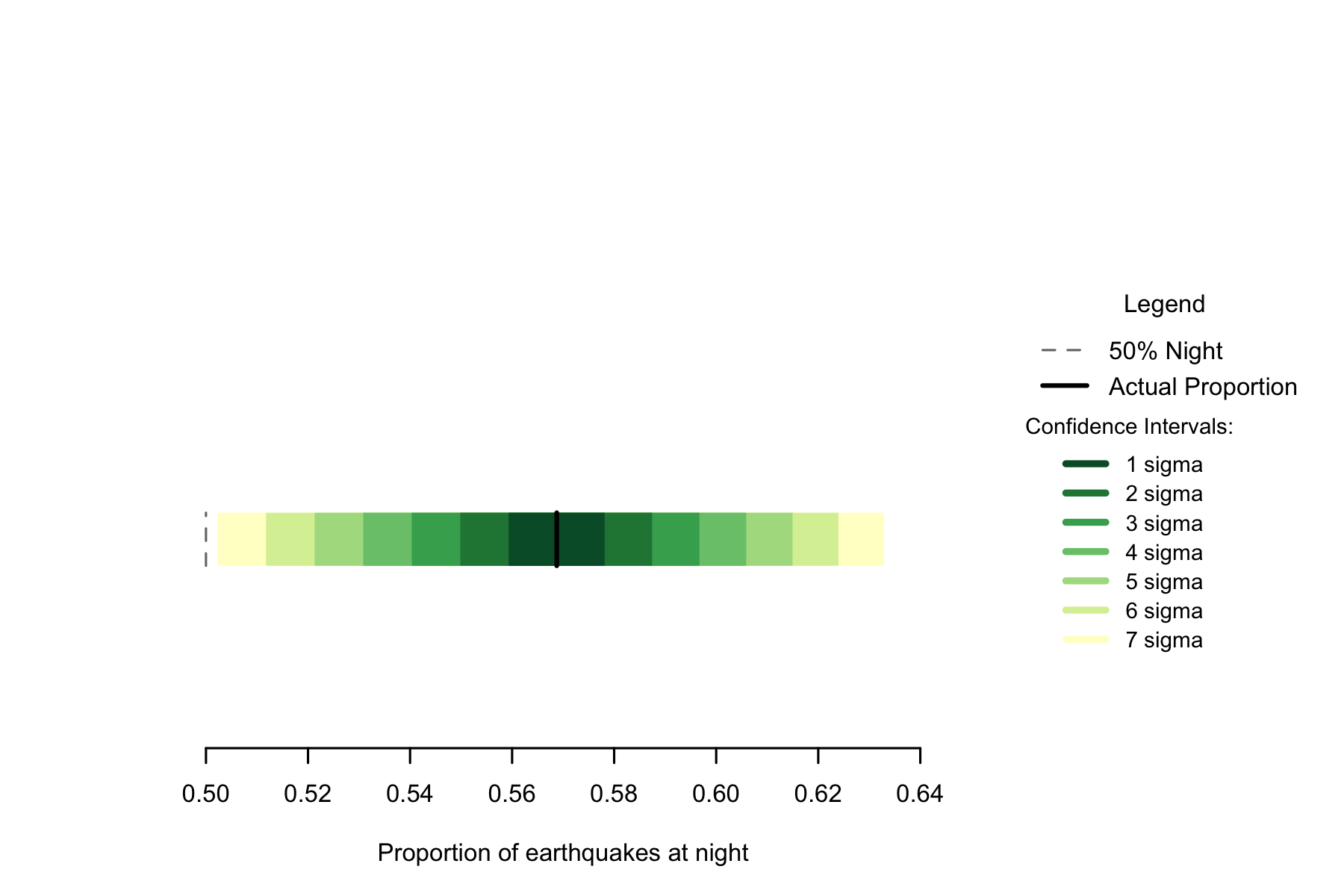
Figure 7.1: Proportion of earthquakes at night: Thailand n=2771
The smaller sample size of the Thai set of data makes wide confidence intervals, but the overall rate is beyond 7 sigma from the expected 0.5 proportion of earthquakes at night
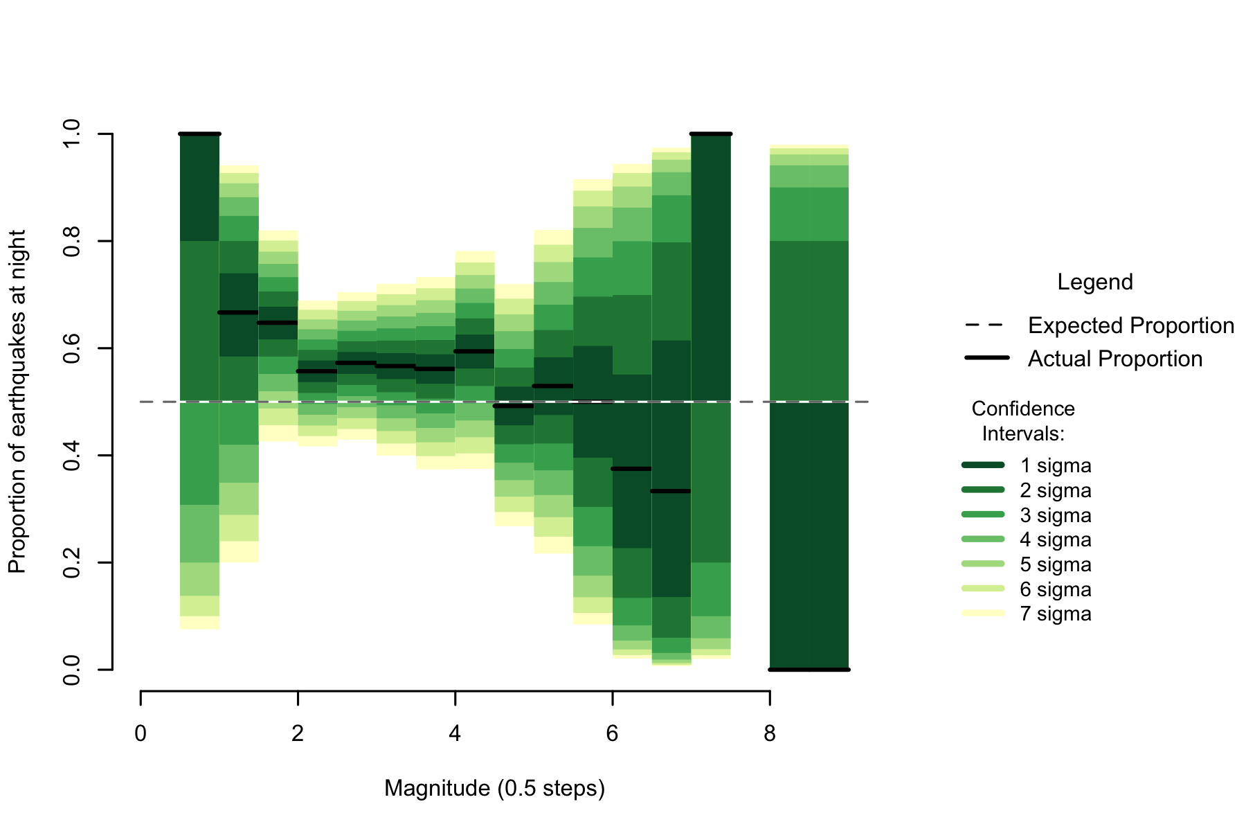
Figure 2.4: Proportion of night earthquakes by magnitude, Thailand n=2771
While there are not enough earthquakes to be certain, the magnitude pattern seems to be similar to the nearby (in global terms) Philippines earthquake data. In the range from magnitude 2 to magnitude 4, where the confidence intervals are smallest, the proportion of night earthquakes seems to be consistently high.
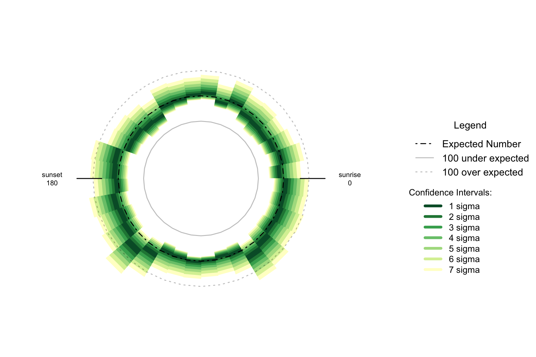
Figure 7.3: Over- and under- supply of earthquakes by angle of the sun (10 degree steps), Thailand n=2771
The trend by angle of the sun also seems similar to the Philippines. There is a generally raised level of earthquake risk at night, with some heightened risk when the sun is 50 to 60 degrees below the horizon. A noticeable decrease in risk occurs as the sun is 30 to 60 degrees above the horizon in the west of the sky.
14.1 Formal Statement
Earthquakes in the region of Thailand show a similar pattern to New Zealand, displaying an oversupply of earthquakes at night that is not the result of chance. While the sample size is to small to make conclusions as confident as the other, larger, datasets, the magnitude patterns are not inconsistent with the general patterns observed in other data sets.
14.2 Links
1 - Thai Meteorological Department, Seismology Bureau http://www.earthquake.tmd.go.th/en/local.php?pageNum_thaievent=106&totalRows_thaievent=4247
14.3 Chapter Code
## ----setup, include=FALSE------------------------------------------------
knitr::opts_chunk$set(echo = FALSE)

## ----c10_001, warnings=FALSE, errors=FALSE, message=FALSE----------------
library(geosphere)
library(lubridate, quietly=TRUE)
library(dplyr)
library(binom)
library(ggplot2)
library(maps)
library(mapdata)
library(parallel)
library(readr)
library(plotrix)
library(tidyr)
library(maptools)
library(rvest)
Sys.setenv(TZ = "UTC")


## ----warnings=FALSE, errors=FALSE, message=FALSE-------------------------


if(!dir.exists("../othereqdata")){
  dir.create("../othereqdata")
}
if(!file.exists("../othereqdata/eq_thailand_raw.RData")){

assemble_eq <- function(x){
  wbpg <- paste("http://www.earthquake.tmd.go.th/en/local.php?pageNum_thaievent=",
                x, "&totalRows_thaievent=4247", sep="")
  th_eq <- read_html(wbpg) %>%
  html_table(header=TRUE)
  return(th_eq[[3]])
  }

eq_list <- lapply(1:105, assemble_eq)
eq_thailand <- bind_rows(eq_list)
names(eq_thailand) <- c("origin_time", "magnitude", "latitude", "longitude", "region")
eq_thailand$time_UTC <- ymd_hms(eq_thailand$origin_time)

eq_national <- eq_thailand %>%
  filter(magnitude >= 0 &
           time_UTC >= as.POSIXct("2011-09-01T00:00:00",
                                  format="%Y-%m-%dT%H:%M:%S", tz="UTC") &
           time_UTC < as.POSIXct("2016-09-01T00:00:00",
                                 format="%Y-%m-%dT%H:%M:%S", tz="UTC")) %>%
  distinct()  %>% arrange(time_UTC)
#one longitude was missing the decimal sign

rm(eq_thailand)
save(eq_national, file="../othereqdata/eq_thailand_raw.RData")
}

## ------------------------------------------------------------------------

if(!file.exists("../othereqdata/eq_thailand_processed.RData")){
load("../othereqdata/eq_thailand_raw.RData")
southmost <- min(eq_national$latitude)
westmost <- min(eq_national$longitude)

eq_national <- eq_national %>% filter(
  magnitude > 0) %>% rowwise() %>% mutate(
  eq_gridpoint_y = round(distVincentyEllipsoid(c(longitude, southmost),
                                               c(longitude,latitude)) /50000,0),
  eq_gridpoint_x = round(distVincentyEllipsoid(c(westmost, latitude),
                                               c(longitude,latitude)) /50000,0),
  eq_roundedlat = destPoint(p=c(longitude, southmost),
                            b=0, d=eq_gridpoint_y*50000)[2],
  eq_roundedlong = destPoint(p=c(westmost, eq_roundedlat),
                             b=90, d=eq_gridpoint_x*50000)[1]) %>% ungroup()
# use maptools to calculate solar angles
sun_angles <- solarpos(matrix(c(eq_national$longitude, eq_national$latitude), ncol=2),
                       eq_national$time_UTC)
colnames(sun_angles) <- c("eq_compass", "eq_vertical")
eq_national <- cbind(eq_national,sun_angles)
eq_national$eq_is_night <- eq_national$eq_vertical < 0
# calculate 360 degree as well as vertical
eq_national <- eq_national %>%
  mutate(eq_angle_360 = eq_vertical,
         eq_angle_360 = ifelse(eq_compass > 180, 180 - eq_angle_360, eq_angle_360),
         eq_angle_360 = ifelse(eq_vertical < 0 & eq_compass <= 180,
                               360 + eq_angle_360, eq_angle_360),
         eq_angle_by_10 = floor(eq_angle_360 /10) * 10)
save(eq_national, file="../othereqdata/eq_thailand_processed.RData")
}

## ------------------------------------------------------------------------
if(!file.exists("../othereqdata/eq_thailand_expected.RData")){
load("../othereqdata/eq_thailand_processed.RData")

lat_range <- unique(eq_national$eq_roundedlat)
long_med <- median(eq_national$eq_roundedlong)

# 1 minute intervals for a full solar year
time1 <- ymd_hms("2015-01-01 00:00:00")
time2 <- ymd_hms("2015-12-31 23:59:00")
time_sq <- seq.POSIXt(from=time1, to=time2, by="min")


calc_angs <- function(x, longinput, timeinput){
  library(dplyr)
  sun_angles <- maptools::solarpos(matrix(c(longinput, x), ncol=2), timeinput)
  colnames(sun_angles) <- c("eq_compass", "eq_vertical")
# calculate 360 degree as well as vertical
site_summary <- as.data.frame(sun_angles) %>%
  mutate(eq_angle_360 = eq_vertical,
         eq_angle_360 = ifelse(eq_compass > 180, 180 - eq_angle_360, eq_angle_360),
         eq_angle_360 = ifelse(
           eq_vertical < 0 & eq_compass <= 180, 360 + eq_angle_360, eq_angle_360),
         eq_angle_by_10 = floor(eq_angle_360 /10) * 10) %>%
  group_by(eq_angle_by_10) %>% summarise(total= n())
  site_summary$lat <- x
  return(site_summary)
}
###
# Calculate the number of cores
no_cores <- detectCores() - 1
# Initiate cluster
cl <- makeCluster(no_cores)
clusterExport(cl, varlist=c("lat_range", "long_med", "time_sq", "calc_angs"))
list_angs <- parLapply(cl, lat_range,
                         function(x){
                           calc_angs(x=x, longinput=long_med, timeinput=time_sq)})
stopCluster(cl)
###
library(tidyr)
anglong <- bind_rows(list_angs)
angwide <- spread(anglong, key=eq_angle_by_10,value=total)
rm(anglong, list_angs, time_sq)
save(angwide, file="../othereqdata/eq_thailand_expected.RData")
}

## ------------------------------------------------------------------------
load("../othereqdata/eq_thailand_processed.RData")
load("../othereqdata/eq_thailand_expected.RData")
eq_night = sum(eq_national$eq_is_night)
eq_total = nrow(eq_national)
 bands <- rev(c('#ffffcc','#d9f0a3','#addd8e','#78c679','#41ab5d','#238443','#005a32'))
 sigmas <- c(0.682689492137086,
 0.954499736103642,
 0.997300203936740,
 0.999936657516334,
 0.999999426696856,
 0.999999998026825,
 0.999999999997440)
 lbls <- c(
 "1 sigma", "2 sigma",
 "3 sigma", "4 sigma",
 "5 sigma", "6 sigma",
 "7 sigma")
typs <- c(1,1,1,1,1,1,1)
weights <- c(3,3,3,3,3,3,3)
old_par=par()

## ------------------------------------------------------------------------
bt <- binom.test(eq_night ,eq_total, conf.level= .999999999997440)

## ------------------------------------------------------------------------
feature <- c("Earliest (UTC)", "Latest (UTC)",
             "Northernmost", "Southernmost",
             "Westmost", "Eastmost",
             "Percent < Mag 3", "total entries",
             "nighttime quakes")
value <- c(as.character(min(eq_national$time_UTC)),
           as.character(max(eq_national$time_UTC)),
           as.character(max(eq_national$latitude)),
           as.character(min(eq_national$latitude)),
           as.character(min(eq_national$longitude)),
           as.character(max(eq_national$longitude)),
           as.character(round(100*sum(eq_national$magnitude < 3)/eq_total,2)),
           as.character(eq_total),
           as.character(eq_night))
data.frame(feature,value) %>% knitr::kable(caption="Data description")

## ---- fig.cap="Proportion of earthquakes at night: Thailand n=2771"------
### making the basic proportion graph
eq_night = sum(eq_national$eq_is_night)
eq_total = nrow(eq_national)
bands <- rev(c('#ffffcc','#d9f0a3','#addd8e','#78c679','#41ab5d','#238443','#005a32'))
sigmas <- c(0.682689492137086,
            0.954499736103642,
            0.997300203936740,
            0.999936657516334,
            0.999999426696856,
            0.999999998026825,
            0.999999999997440)
lbls <- c(
  "1 sigma", "2 sigma",
  "3 sigma", "4 sigma",
  "5 sigma", "6 sigma",
  "7 sigma")
typs <- c(1,1,1,1,1,1,1)
weights <- c(3,3,3,3,3,3,3)
old_par=par()
conf_steps <- function(x, sigmas=sigmas, night=eq_night, total=eq_total){
  ci_lower <- binom.confint(night, total, method=c("wilson"), conf.level = sigmas[x])[1,5]
  ci_upper <- binom.confint(night, total, method=c("wilson"), conf.level = sigmas[x])[1,6]
  ci_data <- data.frame(step = x, ci_lower, ci_upper)
}

ci_spacing <- lapply(7:1, conf_steps, sigmas=sigmas, night=eq_night, total=eq_total)
ci_steps <- bind_rows(ci_spacing)

layout(matrix(c(1,1,1,2), ncol=4))

par(mar=c(5,6,4,2))
plot(c(min(0.5,floor(100*ci_steps[1,2])/100), max(0.5,ceiling(100*ci_steps[1,3])/100)),
       y=c(-3,8), type="n", bty="n", yaxt="n", ylab="",
       xlab="Proportion of earthquakes at night")
a <- a <- apply(ci_steps, 1, function(x){
  polygon(c(x[2], x[3], x[3], x[2]), c(0, 0, 1, 1), col=bands[x[1]], border=NA)})
lines(c(.5,.5), c(0,1), col="#FFFFFF")
lines(c(.5,.5), c(0,1), lty=2, col="#777777")
lines(c(eq_night/eq_total,eq_night/eq_total), c(0,1), lwd=2)

par(mar=c(0,0,0,0))
plot(x=c(0,10), y=c(0,10), type="n", bty="n", axes=FALSE)
legend(0,5.5, legend=lbls, lty=typs, lwd=weights, col=bands, bty="n", xjust=0,
       title="Confidence Intervals:", y.intersp=1.1, cex=0.9)

lbls2=c("50% Night", "Actual Proportion")
typs2=c(2,1)
weights2=c(1,2)
cls2=c("#777777","#000000")
legend(0,7, legend=lbls2, lty=typs2, lwd=weights2, col=cls2, bty="n", xjust=0,
       title="Legend", y.intersp=1.2)


par(mar=old_par$mar)
par(mfrow=c(1,1))


## ---- fig.cap="Proportion of night earthquakes by magnitude, Thailand n=2771"----
old_par=par()
grf <- eq_national %>% mutate(floored_mag = floor(magnitude*2)/2) %>%
  group_by(floored_mag) %>% summarise(successes = sum(eq_is_night), trials=n())

poly_conf_int <- function(success, trials, aa, stepsize, sigma, colr){
  ci <- binom.confint(success, trials, method=c("wilson"), conf.level = sigma)
  lower <- ci[1,5]
  upper <- ci[1,6]
  a <- polygon(x=c(aa,aa+stepsize,aa+stepsize,aa), y=c(upper,upper,lower,lower),
               col=colr, border=NA)
}


plot7sig <- function(success, trials, aa, stepsize){
  library(binom)
  #bands <- c('#ffffb2','#fed976','#feb24c','#fd8d3c','#fc4e2a','#e31a1c','#b10026')
  bands <- rev(c('#ffffcc','#d9f0a3','#addd8e','#78c679','#41ab5d','#238443','#005a32'))
  sigmas <- c(0.682689492137086,
              0.954499736103642,
              0.997300203936740,
              0.999936657516334,
              0.999999426696856,
              0.999999998026825,
              0.999999999997440)
  sapply(7:1, function(x){
    poly_conf_int(success, trials, aa, stepsize, sigmas[x], bands[x])})
  a <- lines(c(aa, aa + stepsize), c(success/trials, success/trials), lwd=2)
}


lbls <- c(
  "1 sigma", "2 sigma",
  "3 sigma", "4 sigma",
  "5 sigma", "6 sigma",
  "7 sigma")
typs <- c(1,1,1,1,1,1,1)
weights <- c(3,3,3,3,3,3,3)
clrs <- rev(c('#ffffcc','#d9f0a3','#addd8e','#78c679','#41ab5d','#238443','#005a32'))
#clrs <- c('#ffffb2','#fed976','#feb24c','#fd8d3c','#fc4e2a','#e31a1c','#b10026')

layout(matrix(c(1,1,1,2), ncol=4))
plot(x=c(0,max(grf$floored_mag)+0.5), y=c(0,1), type="n", bty="n",
     xlab="Magnitude (0.5 steps)", ylab="Proportion of earthquakes at night")
a <- apply(grf,1,function(x){plot7sig(x[2],x[3],x[1],0.5)})
lines(c(0,10), c(.5,.5), col="#FFFFFF")
lines(c(0,10), c(.5,.5), lty=2, col="#777777")

par(mar=c(0,0,0,0))
plot(x=c(0,10), y=c(0,10), type="n", bty="n", axes=FALSE)
legend(0,5, legend=lbls, lty=typs, lwd=weights, col=clrs, bty="n", xjust=0,
       title="Confidence
Intervals:", cex=0.9)
lbls=c("Expected Proportion", "Actual Proportion")
typs=c(2,1)
weights=c(1,2)
legend(0,7, legend=lbls, lty=typs, lwd=weights, bty="n", xjust=0,
       title="Legend", y.intersp=1.2)


par(mar=old_par$mar)
par(mfrow=c(1,1))


## ------------------------------------------------------------------------
by_angle <- eq_national %>%
  group_by(eq_angle_by_10) %>% summarise(total= n()) %>%
  mutate(daynight=ifelse(eq_angle_by_10 < 180, "day", "night"))

merged <- merge(eq_national, angwide, by.x="eq_roundedlat", by.y="lat")
agg_expected <- merged %>% select(`0`:`350`) %>% colSums(na.rm=TRUE)
expected_prop <- agg_expected / sum(agg_expected)
expected <- data.frame(eq_angle_by_10 = as.numeric(names(expected_prop)),
                       expected_prop = as.numeric(expected_prop))
expected$expected_number = expected_prop * eq_total
act_exp <- merge(expected, by_angle, by="eq_angle_by_10", all.x=TRUE)

act_exp$total[is.na(act_exp$total)] <- 0
act_exp$daynight <- NULL
act_exp$act_prop <- act_exp$total / sum(act_exp$total)


ci_brackets <- act_exp %>% ungroup() %>% mutate(grand_total=sum(total)) %>%
  rowwise() %>% mutate(
    ci_lower_7 = binom.confint(total, grand_total, method=c("wilson"),
                               conf.level = sigmas[7])[1,5] * grand_total,
    ci_upper_7 = binom.confint(total, grand_total, method=c("wilson"),
                               conf.level = sigmas[7])[1,6] * grand_total,
    ci_lower_6 = binom.confint(total, grand_total, method=c("wilson"),
                               conf.level = sigmas[6])[1,5] * grand_total,
    ci_upper_6 = binom.confint(total, grand_total, method=c("wilson"),
                               conf.level = sigmas[6])[1,6] * grand_total,
    ci_lower_5 = binom.confint(total, grand_total, method=c("wilson"),
                               conf.level = sigmas[5])[1,5] * grand_total,
    ci_upper_5 = binom.confint(total, grand_total, method=c("wilson"),
                               conf.level = sigmas[5])[1,6] * grand_total,
    ci_lower_4 = binom.confint(total, grand_total, method=c("wilson"),
                               conf.level = sigmas[4])[1,5] * grand_total,
    ci_upper_4 = binom.confint(total, grand_total, method=c("wilson"),
                               conf.level = sigmas[4])[1,6] * grand_total,
    ci_lower_3 = binom.confint(total, grand_total, method=c("wilson"),
                               conf.level = sigmas[3])[1,5] * grand_total,
    ci_upper_3 = binom.confint(total, grand_total, method=c("wilson"),
                               conf.level = sigmas[3])[1,6] * grand_total,
    ci_lower_2 = binom.confint(total, grand_total, method=c("wilson"),
                               conf.level = sigmas[2])[1,5] * grand_total,
    ci_upper_2 = binom.confint(total, grand_total, method=c("wilson"),
                               conf.level = sigmas[2])[1,6] * grand_total,
    ci_lower_1 = binom.confint(total, grand_total, method=c("wilson"),
                               conf.level = sigmas[1])[1,5] * grand_total,
    ci_upper_1 = binom.confint(total, grand_total, method=c("wilson"),
                               conf.level = sigmas[1])[1,6] * grand_total)

norm_ci <- ci_brackets

for (i in c(4,7:20)){
norm_ci[,i] <- ci_brackets[,i] - ci_brackets[,3]
}
circlesize=100

## ---- fig.cap="Over- and under- supply of earthquakes by angle of the sun
## (10 degree steps), Thailand n=2771"----
norm_ci$border = 2
# need to double entries with a displacement of 10
# to make each side of the item on the graph
norm_ci2 <- norm_ci
norm_ci2$eq_angle_by_10 <- norm_ci2$eq_angle_by_10  + 10
norm_ci2$border = 1
graphdata <-   bind_rows(norm_ci,norm_ci2) %>% arrange(eq_angle_by_10,border)

#### plot graph
bands <- rev(c('#ffffcc','#d9f0a3','#addd8e','#78c679','#41ab5d','#238443','#005a32'))
old_par=par()
layout(matrix(c(1,1,1,2), ncol=4))

# overall limits
limits=2 * max(abs(c(graphdata$ci_lower_7, graphdata$ci_upper_7)))
# plot upper confidence 7 interval using plotrix
polar.plot(graphdata$ci_upper_7, polar.pos=graphdata$eq_angle_by_10,
           radial.lim=c(-1*limits,limits),
           labels = "", main=NULL,lwd=0.5, rp.type="p",
           show.grid.labels=FALSE, show.grid=FALSE, mar=c(0,0,0,0),
           grid.col=bands[7], line.col=bands[7], poly.col=bands[7])
# plot upper 6 confidence interval
plot_ci_round <- function(upper_bound,x){
  polar.plot(upper_bound, polar.pos=graphdata$eq_angle_by_10, add=TRUE,
             radial.lim=c(-1*limits,limits),
             line.col=bands[x], lwd=0.5, rp.type="p", poly.col=bands[x])
}
plot_ci_round(graphdata$ci_upper_6, 6)
plot_ci_round(graphdata$ci_upper_5, 5)
plot_ci_round(graphdata$ci_upper_4, 4)
plot_ci_round(graphdata$ci_upper_3, 3)
plot_ci_round(graphdata$ci_upper_2, 2)
plot_ci_round(graphdata$ci_upper_1, 1)
plot_ci_round(graphdata$ci_lower_1, 2)
plot_ci_round(graphdata$ci_lower_2, 3)
plot_ci_round(graphdata$ci_lower_3, 4)
plot_ci_round(graphdata$ci_lower_4, 5)
plot_ci_round(graphdata$ci_lower_5, 6)
plot_ci_round(graphdata$ci_lower_6, 7)
polar.plot(graphdata$ci_lower_7, polar.pos=graphdata$eq_angle_by_10,
           add=TRUE, radial.lim=c(-1*limits,limits),
           line.col="white", lwd=0.5, rp.type="p", poly.col="white")

# plot expected guide line
polar.plot(rep(0,nrow(graphdata)), polar.pos=graphdata$eq_angle_by_10, add=TRUE,
           radial.lim=c(-1*limits,limits),
           rp.type="p", lty=4)
# plot 500 less than expected guide line
polar.plot(rep(-1 * circlesize,nrow(graphdata)), polar.pos=graphdata$eq_angle_by_10,
           add=TRUE,radial.lim=c(-1*limits,limits),
           rp.type="p", lty=1, line.col="#00000044")
# plot 500 more than expected guide line
polar.plot(rep(circlesize,nrow(graphdata)), polar.pos=graphdata$eq_angle_by_10,
           add=TRUE,radial.lim=c(-1*limits,limits),
           rp.type="p", lty=3, line.col="#00000044")

lines(c(-1.5,-1.2)*limits, c(0,0))
lines(c(1.5,1.2)*limits, c(0,0))
text(-1.8*limits,0, label="sunset
180", cex=0.7)
text(1.8*limits,0, label="sunrise
0", cex=0.7)


par(mar=c(0,0,0,0))
plot(x=c(0,10), y=c(0,10), type="n", bty="n", axes=FALSE, xlab="")
lbls <- c(
  "1 sigma", "2 sigma",
  "3 sigma", "4 sigma",
  "5 sigma", "6 sigma",
  "7 sigma")
typs <- c(1,1,1,1,1,1,1)
weights <- c(3,3,3,3,3,3,3)
clrs <- rev(c('#ffffcc','#d9f0a3','#addd8e','#78c679','#41ab5d','#238443','#005a32'))
legend(0,4.5, legend=lbls, lty=typs, lwd=weights, col=clrs, bty="n", xjust=0,
       title="Confidence Intervals:", cex=0.9)

lbls2=c("Expected Number", paste(circlesize,"under expected"),
        paste(circlesize,"over expected"))
typs2=c(4,1,3)
weights2=c(1,1,1)
clrs2=c("#000000","#00000044","#00000044")
legend(0,10, legend=lbls2, lty=typs2, lwd=weights2, bty="n", xjust=0,
       title="Legend", y.intersp=1.2, col=clrs2)


par(mar=old_par$mar)
par(mfrow=c(1,1))